Int. J. Communications, Network and System Sciences, 2011, 4, 180-188
doi:10.4236/ijcns.2011.43022 Published Online March 2011 (http://www.SciRP.org/journal/ijcns)
Krige Method Application for the Coverage Analysis of a
Node-B in a WCDMA Network
Jazmín Ponce-Rojas, Sergio Vidal-Beltrán, José Luis López-Bonilla, Montserrat Jimenez-Licea
Maestría en Ciencias en Ingeniería de Telecomunicaciones, Escuela Superi or de In ge ni erí a Mec áni c a y Eléct ri ca,
Instituto Politécnico Nacional, México City, México
Received January 17, 2011; revised February 19, 2011; accepted February 21, 2011
Abstract
This paper shows the procedure and application of the Krige Method (or Kriging) for the analysis of the
power level radiated by a Base Station (also called Node B), through a group of samples of this power level,
measured at different positions and distances. These samples were obtained using an spectrum analyzer,
which will allow to have georeferenced measurements, to implement the interpolation process and generate
coverage maps, making possible to know the power level distribution and therefore understand the behavior
and performance of the Node B.
Keywords: Interpolation, Krige, Node B, WCDMA
1. Introduction
At the present time WCDMA (Wideband Code Division
Multiple Access) is a medium access technique imple-
mented in many countries around the world, including
Mexico. This technique allows the user to occupy the
entire bandwidth in any time, because identifying infor-
mation of each mobile station through codes, allowing
reliable transmission within the same channel not sepa-
rated in time or frequency. WCDMA provides high trans-
fer rates, efficient support of asymmetric traffic, transmis-
sion using packet switching through the radio interface
and high efficiency in spectrum use.
The Base Station (BS), also known as Node B, is part
of the UMTS Terrestrial Radio Access Network (UTRAN).
The Node B has as main tasks make the transmission and
reception of radio signal, filtering of the signal, amplifi-
cation, modulation and demodulation of the signal and be
an interface to the Radio Network Controller (RNC) [1].
The Common Pilot Channel (CPICH) transmits a carrier
used to estimate the channel parameters; is the physical
reference for other channels. It is used to control power,
consistent transmission and detection, cannel estimation,
measurement of adjacent cells and obtaining of the Scram-
bling Code (SC) [2].
The Krige Method is an interpolation technique based
in a sample regression, which are irregularly spaced, to
predict unknown values from known values. It is a fam-
ily of generalized algorithms for least squares that from a
set of observations provides the optimal linear predictor
for the variable in any position.
This method was developed by Daniel G. Krige in an
attempt to predict more accurately the mineral reserves.
In recent decades the Krige Method has become a fun-
damental tool in the field of the geostatistics because
founded the basis of linear geostatistical. It is a geostatis-
tical method for estimating points that using a variogram
model to obtain data. It is based on the premise that the
spatial variation continues with the same pattern.
The variogram or semivariogram is a tool that allows
analyzes the spatial behavior of a variable on a defined
area, resulting in the influence of data at different dis-
tances. From the data provided by the theoretical vario-
gram the estimation is performed by the method of Krige.
The semivariogram is a measure of how similar is the
points in the space when they are farther apart. To de-
velop a variogram first requires creating an experimental
variogram based on the selected simple, and choose a
theoretical variogram that fit the experimental, because
this is not a function where we can make interpolations.
The spatial variations correlated are treated in func-
tions as the variogram, which show the information to
optimize the weights and choose radios precise data
search. Known the variogram and the original observa-
tions, you can get a set of achievements to show the
range of possible values.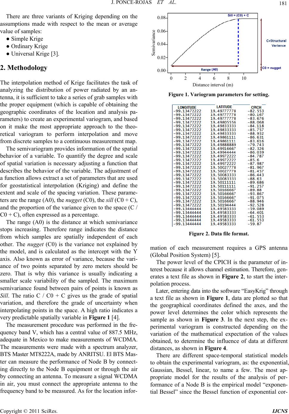

J. PONCE-ROJAS ET AL.
181
There are three variants of Kriging depending on the
assumptions made with respect to the mean or average
value of samples:
● Simple Krige
● Ordinary Krige
● Universal Krige [3].
2. Methodology
The interpolation method of Krige facilitates the task of
analyzing the distribution of power radiated by an an-
tenna, it is sufficient to take a series of grab samples with
the proper equipment (which is capable of obtaining the
geographic coordinates of the location and analysis pa-
rameters) to create an experimental variogram, and based
on it make the most appropriate approach to the theo-
retical variogram to perform interpolation and move
from discrete samples to a continuous measurement map.
The semivariogram provides information of the spatial
behavior of a variable. To quantify the degree and scale
of spatial variation is necessary adjusting a function that
describes the behavior of the variable. The adjustment of
a function allows extract a set of parameters that are used
for geostatistical interpolation (Kriging) and define the
extent and scale of the spacing variation. These parame-
ters are the range (A0), the nugget (C0), the sill (C0 + C),
and the proportion of the variance given to the space (C /
C0 + C), often expressed as a percentage.
The range (A0) is the distance at which semivariance
stops increasing. Therefore range indicates the distance
from which samples are spatially independent of each
other. The nugget (C0) is the variance not explained by
the model, and is calculated as the intercept with the Y
axis. Also known as error of variance, because the vari-
ance of two points separated by zero meters should be
zero. That is why this variance is usually indicating a
smaller scale variability of the sampled. The maximum
semivariance found between pairs of points is known as
Sill. The ratio C / C0 + C gives us the grade of spatial
variation, and therefore the grade of uncertainty when
interpolating points in the space. A high ratio indicates a
very predictable spatially variable in Figure 1 [4].
The measurement procedure was performed in the fre-
quency band V, which has a central value of 887.5 MHz,
adequate in Mexico to make measurements of WCDMA.
The measurements were made with a spectrum analyzer,
BTS Master MT8222A, made by ANRITSU. El BTS Mas-
ter can measure the performance of Node B by connect-
ing directly to the Node B equipment or through the air
by connecting an antenna. To measure a signal WCDMA
in air, you must connect the appropriate antenna to the
frequency band to be measured. As for the location infor-
Distance interval (m)
Semivariance
0 2 4 6 8 10
0.08
0.00
0.02
0.04
0.06
(A0)
Sill = (C0) + C
C0 = nugget
Figure 1. Variogram parameters for setting.
Figure 2. Data file format.
mation of each measurement requires a GPS antenna
(Global Position System) [5].
The power level of the CPICH is the parameter of in-
terest because it allows channel estimation. Therefore, gen-
erates a text file as shown in Figure 2, to start the inter-
polation process.
Later, entering data into the software “EasyKrig” through
a text file as shown in Figure 1, data are plotted so that
the geographical coordinates defined the axes, and the
power level determines the color which represents the
sample as shown in Figure 3. In the next step, the ex-
perimental variogram is constructed depending on the
variation of the mathematical expectation of the values
obtained, to determine the influence of data at different
distances, as shown in Figure 4.
There are different space-temporal statistical models
to obtain the experimental variogram, as: the exponential,
Gaussian, Bessel, linear, to name a few. The most ap-
propriate model for the results of the analysis of per-
formance of a Node B is the empirical model “exponen-
tial Bessel” since the Bessel function of exponential cor-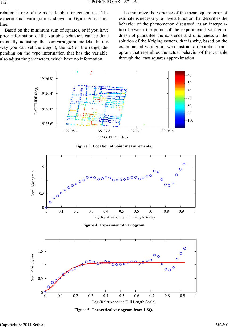

J. PONCE-ROJAS ET AL.
182
To minimize the variance of the mean square error of
estimate is necessary to have a function that describes the
behavior of the phenomenon discussed, as an interpola-
tion between the points of the experimental variogram
does not guarantee the existence and uniqueness of the
solution of the Kriging system, that is why, based on the
experimental variogram, we construct a theoretical vari-
ogram that resembles the actual behavior of the variable
through the least squares approximation.
relation is one of the most flexible for general use. The
experimental variogram is shown in Figure 5 as a red
line.
Based on the minimum sum of squares, or if you have
prior information of the variable behavior, can be done
manually adjusting the semivariogram models. In this
way you can set the nugget, the sill or the range, de-
pending on the type information that has the variable,
also adjust the parameters, which have no information.
LONGITUDE (deg)
–
40
–
50
–
60
–
70
–
80
–
90
–
100
–
99˚08.4'
–
99˚07.8'
–
99˚07.2'
–
99˚06.6'
19˚26.8'
19˚26.4'
19˚26.0'
19˚25.6'
LATITUDE (deg)
Figure 3. Location of point measurements.
Lag (Relative to the Full Length Scale)
0 0.1 0.2 0.3 0.4 0.5 0.6 0.7 0.8 0.9 1
Semi-Variogram
1.5
1
0.5
0
Figure 4. Experimental variogram.
Lag (Relative to the Full Length Scale)
0
0.1 0.2 0.3 0.4 0.5 0.6 0.7 0.8 0.9 1
Semi-Variogram
1.5
1
0.5
0
Figure 5. Theoretical variogram from LSQ.

J. PONCE-ROJAS ET AL.
183
The Figure 6 is obtained using Ordinary Krige, be-
cause the mean value is not known, and we know that the
value is not constant throughout the study area, but lo-
cally can be considered constant; because measurements
are made at a distance will be very similar to those made
in the vicinity of that point.
Finally, it makes the validation step shown in Figure 7,
to be sure that the mean square error is within the accep-
tance region to eliminate any doubt with respect to reli-
ability, efficiency, consistency, sufficiency and unbiased-
ness of the power level estimator for proper analysis of
the performance of a Node B.
3. Results
As a statistical method each map generation to will be as
different as theoretical variograms can be constructed.
Obviously, this will depend on the behavior of data.
When making a large number of samples concentrated in
a given space, as is shown in Figure 8, has a behavior
which is very close to the experimental way, as is shown
in Figure 9.
Consequently, the approximation error Q will be very
small and is within the expected range in the Gaussian
bell, as shown in Figure 7.
LONGITUDE (deg)
–
50
–
60
–
70
Figure 6. Coverage map.
Q
1
–
0.25 –0.2 –0.15 –0.1 –0.05 0 0.05 0.1 0.15 0.2 0.25
10
9
8
7
6
5
4
3
2
1
0
PDF(Q
1
)
Accept Region
Computed Q
1
Q
1
=
–
0.00710802
Figure 7. Validation of the interpolation process.
LONGITUDE
(
de
g)
–
50
–
60
–
70
–
80
–
90
–
99˚08.4'
–
99˚08.2'
–
99˚08 .0'
–
99˚07.8'
19˚30.2'
19˚30.0'
19˚29.8'
LATITUDE (deg)
Figure 8. Location of 592 samples.
–
90
–
99°08.4'
–
99°08.0'
–
99°07.6'
–
99°07.2'
19°26.8'
19°26.4'
19°26.0'
19°25.6'
LATITUDE (deg)
–
55
–
65
–
80
–
75
–
85

184 J. PONCE-ROJAS ET AL.
When preset conditions are met, coverage map is
properly constructed (Figure 6), and therefore is very
clear assessment of the location of the Base Station, the
obstacles to the propagation, the attenuation of the signal
as a function of distance, the area in which the received
signal is reasonably good.
Then there were three cases showing variations in the
results.
In the first case were obtained 592 point samples, with
a minimum value of power level of –95.9 dBm and
maximum power measurement of –43.8 dBm. The dis-
tribution of these measurements is shown in Figure 8.
The greatest concentration is in the center of the study
area, therefore be as nearby the power values measured
do not vary drastically.
Although the range between the highest and the lowest
power levels very ample, the large number of samples
allows have a semivariogram with a fairly predictable
behavior, and therefore adjust the theoretical semivario-
gram, as shown in Figure 9.
The efficiency of the estimate is checked through the
validation process, getting the error of approximation Q
is within the acceptance region as shown in Figure 10.
Having a large number of samples is achieved that the
area where the coverage map applies is very similar to
the total test area as is shown in Figure 11.
If the samples are few, but are concentrated in a spe-
cific area of the measuring area, is possible to obtain
reliable results, but only within that space, as shown in
Figure 15, coordinates have smaller increments, because
the data provided are sufficient to know only the power
level in the vicinity of the points. Locate the Base Station
is not an easy task as it is not the interpretation of the
maps. This case is illustrated in Figures 12 to 15.
For this case were obtained 120 samples, with maximum
power level of –69.5 dBm and a minimum of –97.9 dBm.
The distribution of samples is more irregular as shown in
Figure 12.
Due of the greater distance between samples the simi-
larity between them is less and therefore adjustment of
the experimental semivariogram is more difficult as shown
in Figure 13.
The approximation error is greater than in the previous
case but is in the region of acceptance as shown in Fig-
ure 14.
Lag (Relative to the Full Length Scale)
0
0.1 0.2 0.3 0.4 0.5 0.6 0.7 0.8 0.9 1
Semi-Variogram
1.5
1
0.5
0
2
2.5
3
Figure 9. Setting theoretical semivariogram to experimental for 592 samples.
Accept Region
Computed Q
1
Q
1
= 0.0440975
Q
1
–
0.4 –0.3 –0.2 –0.1 0 0.1 0.2 0.3 0.4
6
5
4
3
2
1
0
PDF(Q
1
)
Figure 10. Validation procedures for 592 samples.

J. PONCE-ROJAS ET AL.
185
LONGITUDE (deg)
–
60
–
70
–
99˚08.2'
–
99˚08.0'
19˚30.0'
19˚29.8'
LATITUDE (deg)
–
55
–
65
–
80
–
75
–
85
Color Scale
Figure 11. Coverage map for 592 samples.
LONGITUDE (deg)
–
70
–
80
–
90
–
99˚08.2 '
–
99˚08.0'
19˚30.2'
19˚30.0'
LATITUDE (deg)
–
75
–
85
–
95
Figure 12. Location of 120 measurements.
Lag (Relative to the Full Length Scale)
0 0.1 0.2 0.3
0.4 0.5 0.6 0.7 0.8 0.9 1
Semi-Variogram
1.5
1
0.5
0
2
2.5
Figure 13. Semivariogram adjustment from theoretical to experimental (120 samples).
Accept Region
Computed Q
1
Q
1
= 0.159873
Q
1
–
0.8 –0.6 –0.4 –0.2 0 0.2 0.4 0.6
3.5
3
2.5
2
1.5
1
0.5
0
PDF(Q
1
)
Figure 14. Validation process for 120 samples.

J. PONCE-ROJAS ET AL.
186
The area of validity of the interpolation, as expected,
is considerably reduced compared to the total area of
study as shown in Figure 15, due to the smaller number
of samples obtained.
For the third case we have 87 measurements which
minimum power level is –97.634 dBm while the maxi-
mum is –74.697 dBm. The area in which samples are
distributed is far less than the total study areas shown in
Figure 16. What is reflected in the experimental vario-
gram in Figure 17.
However the approximation error Q is minimal; near-
by to zero as seen in Figure 18. This is because the power
range is much smaller than in the previous cases, there-
fore the difference between the powers measured in ad-
jacent points is less reducing the range of possible values
of power at each interpolation.
When the power range is as small as this case is possi-
ble to appreciate the change in the level with more clarity,
but consequently the area of validity of the estimate is
much lower as reflected in the scales of the axes in Fig-
ure 19.
Finally, when the data are barely sufficient to generate
a theoretical variogram and the separation between them
is great, the approximation error will be larger, or some-
times not be in the range of acceptance. When measure-
ments are made at a great distance from the Node B there
can be problems like this, accordingly analysis of the
radiation pattern is more complicated.
LONGITUDE (deg)
–
99.13 8
19.503
LATITUDE (deg)
–
79
Color Scale
–
80
–
81
–
82
–
83
–
84
–
85
–
86
–
87
–
99.13 7
–
99.136
–
99.13 5
–
99.13 4
–
99.13 3
19.502
19.501
19.5
19.499
19.498
Figure 15. Coverage map for 120 samples.
LONGITUDE (deg)
–
80
–
90
–
99˚08.2'
–
99˚08.0'
19˚30.2'
19˚30.0'
LATITUDE (deg)
–
75
–
85
–
95
Figure 16. Location of 87 measurements.
Lag (Relative to the Full Length Scale)
0 0.1 0.2 0.3 0.4 0.5 0.6 0.7 0.8 0.9 1
Semi-Variogram
1.5
1
0.5
0
Figure 17. Semivariogram adjustment from theoretical to experimental (87 samples).

J. PONCE-ROJAS ET AL.
187
Accept Region
Computed Q
1
Q
1
= –0.0148244
Q
1
–
0.8 –0.6 –0.4 –0.2 0 0.2 0.4 0.6 0.8
3
2.5
2
1.5
1
0.5
0
PDF(Q
1
)
Figure 18. Validation process for 87 samples.
LONGITUDE (deg)
–
99.13 8
19. 503
LATITUDE (deg)
–
72
Color Scale
–
99.137
–
99.13 6
–
99.135
–
99.13 4
19. 502
19. 501
19.5
19. 499
19. 498
–
99.13 85
–
99.1345
–
99.13 55
–
99.13 65
–
99.1375
–
74
–
76
–
78
–
80
–
82
–
84
–
86
–
88
–
90
–
92
Figure 19. Coverage map for 87 samples.
4. Conclusions
Based in the results, is possible concluded that the Krige
Method is optimal for power levels analysis in WCDMA,
because from point data can be generated continuous
coverage maps through a process of interpolation which
predicts the power values in places where there is not
information based on adjacent values. To create reliable
coverage maps is necessary to take into account the fol-
lowing considerations.
● Make sure you have a sufficient number of meas-
urements, which will depend on the total area to study
and variable power levels.
● If the power levels are divers, nearby samples allow
greater similarity exists between them and ensures that
the interpolation will be more reliable in an area very
similar to the total.
● Although it is possible to validate a coverage map
with a smaller number of samples, this will depend on
the operating conditions of the Node B.
● If the level is very variable in the measurement area
measurement should be taken as nearby as possible,
make sure the position information change, otherwise
only have many power values at the same point and it
will be unnecessary information for the estimation proc-
ess.
● If the power levels are not drastic changes can be
estimated efficiently without taking a large number of
samples.
● To optimize the computing time, data must be ar-
ranged in descending or ascending primarily based on
the longitude information, later depending on latitude
and finally based on power levels. Taking the same order
for all the columns in which information is organized.
Since the variogram is obtained based on comparisons
between pairs of neighboring points and the smaller the
difference between them narrower the range of possible
power values interpolated between them, obtaining a
more efficient estimation.
● Measurements were made at a height between 1.1
and 1.4 meters since it is the average height in which
users carry mobile devices.
5. Acknowledgements
Authors thank to the IPN for the support received.

188 J. PONCE-ROJAS ET AL.
6. References
[1] K. Tachikawa, “WCDMA Mobile Communications Sys-
tem,” John Wiley & Sons, Hoboken, 2002.
[2] L. Jaana, W. Achim and N. Tomás, “Radio Network
Planning and Optimization for UMTS,” 2nd Edition, John
Wiley and Sons, Hoboken, 2006.
[3] I. Gual, M. Victoria and S. V. Amelia, “Space-Temporal
Models Statistics in Perimetry,” Doctoral Thesis, De-
partment of Mathematics, School of Technology and Ex-
perimental Sciences, Jaume 1 University, Castellón de la
Plana, 2003.
[4] J. I. Z. Castro, “Analysis of Pilot Pollution in WCDMA
Networks,” Masters Thesis, National Polytechnic Insti-
tute, México, 2011.
[5] Practical Tips on WCDMA Measurements, Application
Note No. 11410-00378, Revision B, United States, 2008.