Int. J. Communications, Network and System Sciences, 2011, 4, 147-151
doi:10.4236/ijcns.2011.43018 Published Online March 2011 (http://www.SciRP.org/journal/ijcns)
Optimum Relay Location in Cooperative Communication
Networks with Single AF Relay
Lei Xu, Hong-Wei Zhang, Xiao-Hui Li*, Xian-Liang Wu
The Key Laboratory of Intelligent Computing and Signal Processing, Ministry of Education,
Anhui University, Hefei, China
Received December 12, 2010; revised January 28, 2011; accepted February 3, 2011
Abstract
In recent years cooperative diversity has been widely used in wireless networks. In particular, cooperative
communication with a single relay is a simple, practical technology for wireless sensor networks. In this pa-
per, we analyze several simple network topologies. Under the condition of equal power allocating, the opti-
mum relay location of each network topology are respectively made sure by using symbol error rate (SER)
formula. And these types of topologies are compared, the analysis results show that, linear network topology
has the best system performance, the system performance of isosceles triangle topology is better than that of
equilateral triangle topology.
Keywords: Relay Location, Cooperative Communication, AF (Amplify and Forward), Topology
1. Introduction
Multiple antennas transmitting diversity technology has
been investigated based on their ability to co mbat fading
induced by multi-path of the channel, and has been
widely used in wireless communication system. However,
the deployment of antenna array on mobile terminal is
difficult due to the size and power limitation. In order to
solve this problem a new mode of gaining transmit di-
versity called cooperative diversity has been proposed
and widely studied [1]. The terminals share their anten-
nas and other resources to create a “virtual array” through
distributed transmission and signal processing [2].
Compared with the multi-relay cooperative communi-
cation, single-relay cooperative communication has more
practical value for wireless sensor networks [3]. The re-
search for single-relay cooperative communication net-
work topology has great significance for improving the
performance of cooperative systems. Paper [4] has
pointed out that, the location of relay has an impact on
the performance of the system. However, the analytic
network topology is single and has not given the theo-
retical basis of the optimal relay location. In this paper,
what is mainly concerned is that, in the uncoded coop-
erative communication system, the position of relay is
how to affect the SER performance of the system. Ac-
cording to the SER formula of single-relay cooperative
communication system [5], in several equal-power allo-
cated simple network topologies, the optimal relay loca-
tion is trying to be gotten. The comparison system per-
formance among these types of network topologies will
be done.
2. System Model
The block diagram of single-relay cooperative commu-
nication system is shown as Figure 1.
The mechanism of single-relay cooperative communi-
cation is divided into two stages. Both stages use the
orthogonal channel, such as TDMA, FDMA, or CDMA.
In the first phase, source node sends symbols to the des-
tination node; relay node receives the symbols sent from
source node at the same time. The received symbols ys,d
and ys,r at destination node and relay node, respectively,
can be written as






,1, ,sdsd ssd
yPhnxnzn (1)






,1, ,srsrssr
yPhnxnzn (2)
In which xs[n] is the transmitted information; P1 is the
transmitted power at the source node; hs,d is the channel
coefficients from source n ode to destination node, which
can be written as




,,,sdsd sd
hnd an ,


,sd
an can be
modeled as a zero mean, complex Gaussian random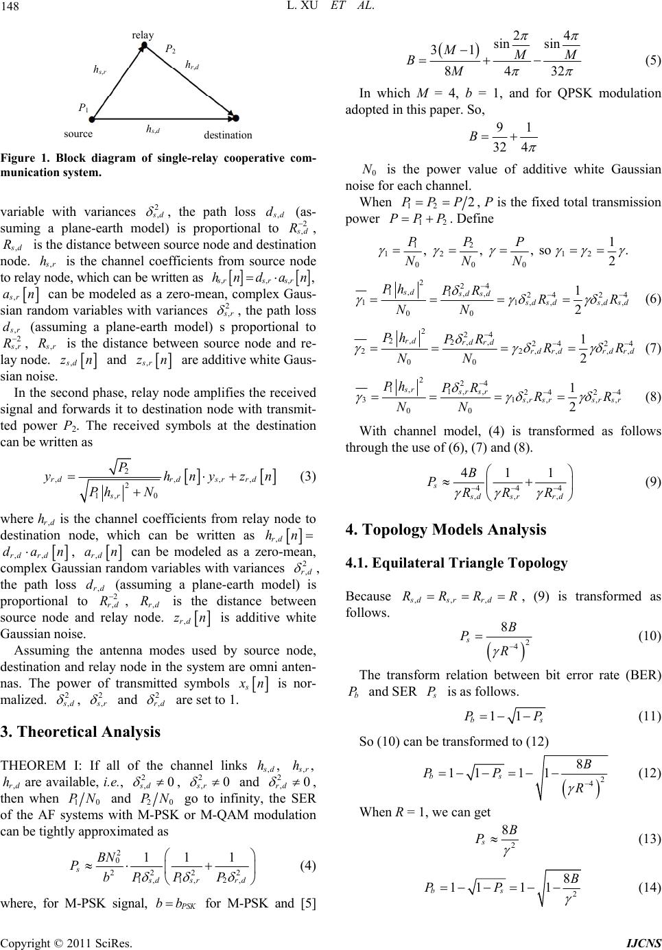

148 L. XU ET AL.
relay
source destination
P
1
P
2
h
s,r
h
s,d
h
r,d
Figure 1. Block diagram of single-relay cooperative com-
munication system.
variable with variances 2
,
s
d

, the path loss ,
s
d
d (as-
suming a plane-earth model) is proportional to 2
,
s
d
R

,
,
s
d
R is the distance between source node and destination
node. ,
s
r
h he channel coefficients from source node
to relay node, which can be written as

is t



,,,
,
srsr sr
hnd an


,sr
an can be modeled as a zero-mean, complex Gaus-
sian random variables with variances 2
,
s
r

, the path loss
,
s
r
d (assua plane-earth modeloportional to
2
,
ming ) s pr
s
r
R, ,
s
r
R is the distance between source nodeand re-
lay node.


,sd
zn and


,sr
zn are additive white
sian Gaus- noise.
In the second phase, relay node amplifies the received
signal and forwards it to destination node with transmit-
ted power P2. The received symbols at the destination
can be written as
 
2
,,,
2
1, 0
rdrdsr rd
sr
P
yhny
Ph N

,
zn (3)
where ,rd
h is the channel coefficients from relay node to
destination node, which can be written as


,rd
hn



,,rd rd, dan 

,rd
an can be modeled as a zero-mean,
complex Gaussian random variables with variances 2
,rd

,
the path loss ,rd (assuming a plane-earth model) is
proportional to , ,rd is the distance between
source node and relay node.
d2
,rd
RR


,rd
zn is additive white
Gaussian nois e.
Assuming the antenna modes used by source node,
destination and relay node in the syste m are omni anten-
nas. The power of transmitted symbols


s
x
n is nor-
malized. 2
,
s
d

, 2
,
s
r

and 2
,rd

are set to 1.
3. Theoretical Analysis
THEOREM I: If all of the channel links ,,
s
d
h ,,
s
r
h0
,rd are available, i.e., , and rd
h2
,0
sd
 2
,0
sr
 2
,


,
then when 10 PN and 20 PN go to infinity, the SER
of the AF systems with M-PSK or M-QAM modulation
can be tightly approximated as
2
0
222 2
1, 1,2,
11 1
s
sd srrd
BN
PbP PP
 

 


(4)
where, for M-PSK signal,
P
SK
bb

for M-PSK and [5]

24
sin sin
31
8432
M
M
M
BM





 (5)
In which M = 4, b = 1, and for QPSK modulation
adopted in this paper. So, 91
32 4
B


0 is the power value of additive white Gaussian
noise for each channel.
N
When 12 2PPP

, P is the fixed total transmission
power 1 PPP
2

. Define
12
12 12
000
1
, , , so .
2
PPP
NNN

    
224
1, 1, ,24 2
11,,
00
1
2
sd sd sd4
,,
s
dsd sdsd
Ph PR RR
NN



   (6)
224
2, 2, ,2424
22,, ,,
00
1
2
rd rd rd
rd rdrd rd
Ph PR RR
NN



   (7)
224
1, 1, ,24 24
31,,,,
00
1
2
sr sr sr
s
rsr srsr
Ph PR RR
NN



  
(8)
With channel model, (4) is transformed as follows
through the use of (6), (7) and (8).
44 4
,, ,
411
s
sd srrd
B
PRR R
 
 





R
(9)
4. Topology Models Analysis
4.1. Equilateral Triangle Topology
Because ,,,sdsr rd RRR

, (9) is transformed as
follows.

2
4
8
s
B
P
R 

 (10)
The transform relation between bit error rate (BER)
and SER
b
P
s
P is as follows.
11
b
Ps P

 (11)
So (10) can be transfo rmed to (12)

2
4
8
11 11
bs
B
PP
R 

   (12)
When R = 1, we can get
2
8
s
B
P

 (13)
2
8
11 11
bs
B
PP

   (14)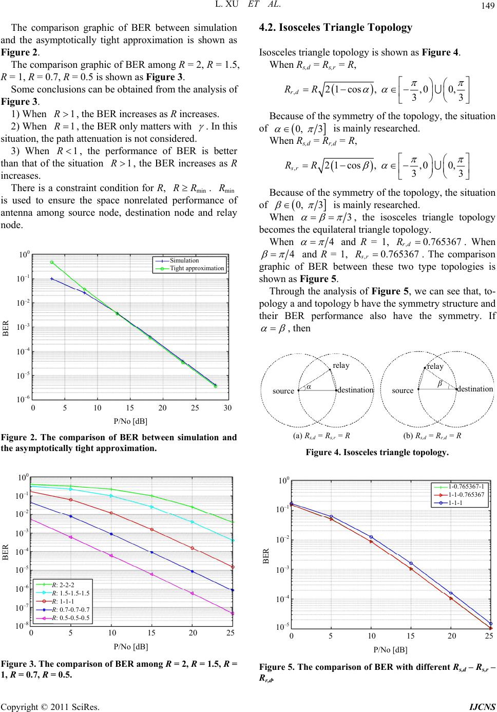

L. XU ET AL.
149
The comparison graphic of BER between simulation
and the asymptotically tight approximation is shown as
Figure 2.
The comparison graphic of BER among R = 2, R = 1.5,
R = 1, R = 0.7, R = 0.5 is shown as Figure 3 .
Some conclusions can be obtained from the analysis of
Figure 3.
1) When , the BER increases as R increases.
1R
2) When , the BER only matters with
1R

. In this
situation, the path attenuatio n is not considered.
3) When , the performance of BER is better
than that of the situation , the BER increases as R
increases.
1R1R
There is a constraint condition for R, .
is used to ensure the space nonrelated performance of
antenna among source node, destination node and relay
node.
min
RRmin R
Simulation
Ti ght approximation
P/No
[
dB
]
0 5 10 15 20 25 30
BER
10
0
10
–1
10
–2
10
–3
10
–4
10
–5
10
–6
Figure 2. The comparison of BER between simulation and
the asymptotically tight approximation.
R
: 2-2-2
R
: 1.5- 1.5-1. 5
R
: 1-1-1
R
: 0.7- 0.7-0. 7
R
: 0.5- 0.5-0. 5
P/No
[
dB
]
0 5 10 15 20 25
BER
10
0
10
–1
10
–2
10
–3
10
–4
10
–5
10
–6
10
–7
10
–8
Figure 3. The comparison of BER among R = 2, R = 1.5, R =
1, R = 0.7, R = 0.5.
4.2. Isosceles Triangle Topology
Isosceles triangle topology is shown as Figure 4.
When Rs,d = Rs,r = R,
 ,21cos, ,00,
33
rd
RR





 
 



Because of the symmetry of the topology, the situation
of


0, 3   is mainly researched.
When Rs,d = Rr,d = R,
 ,21cos, ,00,
33
sr
RR





 
 



Because of the symmetry of the topology, the situation
of


0, 3   is mainly researched.
When 3



, the isosceles triangle topology
becomes the equilateral triangle top ology.
When 4



and R = 1, . When
,0.765367 rd
R
4



and R = 1, ,sr R0.765367

. The comparison
graphic of BER between these two type topologies is
shown as Figure 5.
Through the analysis of Figure 5, we can see that, to-
pology a and topology b have the symmetry structure and
their BER performance also have the symmetry. If



, then
relay relay
source source
destination destination
β
α
(a) Rs,d = Rs,r = R (b) Rs,d = Rr,d = R
Figure 4. Isosceles triangle topology.
P/No
[
dB
]
0 5 10 15 20 25
BER
10
0
10
–1
10
–2
10
–3
10
–4
10
–5
1-0.765367-1
1-1-0.765367
1-1-1
Figure 5. The comparison of BER with different Rs,d – Rs,r –
Rr,d.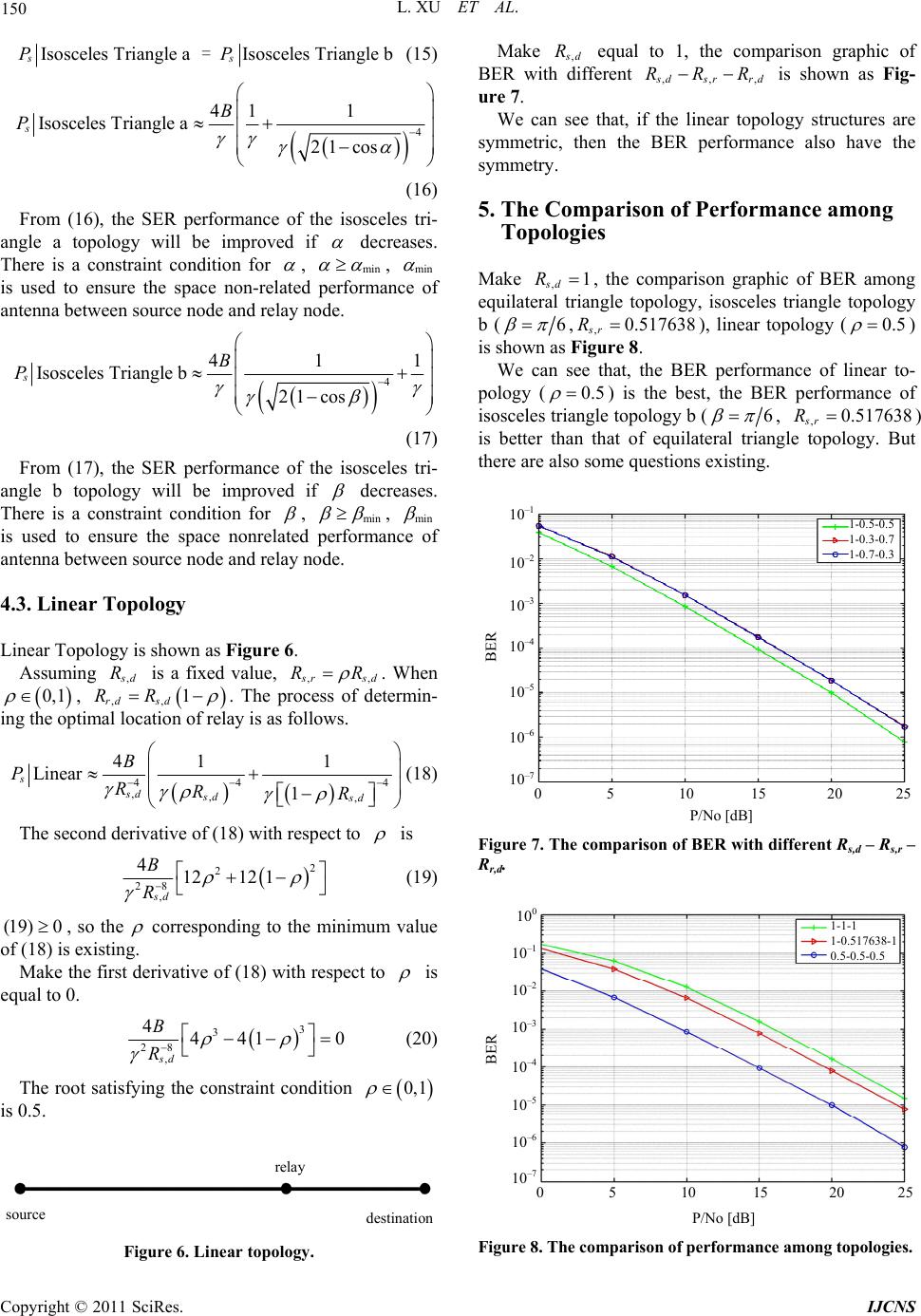

150 L. XU ET AL.
Isosceles Triangle aIsosceles Triangle b
ss
PP = (15)


4
41 1
Isosceles Triangle a21 cos
s
B
P






 




(16)
From (16), the SER performance of the isosceles tri-
angle a topology will be improved if

decreases.
There is a constraint condition for

, min

 , min

is used to ensure the space non-related performance of
antenna betwe en s o urce node and relay node.


4
41
Isosceles Tri angle b21 cos
s
B
P1










(17)
From (17), the SER performance of the isosceles tri-
angle b topology will be improved if

decreases.
There is a constraint condition for

, min

 , min

is used to ensure the space nonrelated performance of
antenna betwe en s o urce node and relay node.
4.3. Linear Topology
Linear Topology is shown as Figure 6.
Assuming ,
s
d
R is a fixed value, ,,
s
r
RR
sd

. When
,

0, 1  

,,
1
sd

rd
RR

. The process of determin-
ing the optimal location of relay is as follows.
 
44
,,,
41 1
Linear 1
s
sd sd sd
B
PRRR
 








4
(18)
The second derivative of (18) with respect to

is

2
2
28
,
41212 1
sd
B
R





 (19)
(19) 0, so the

corresponding to the minimum value
of (18) is existing.
Make the first derivative of (18) with respect to

is
equal to 0.

3
3
28
,
4441
sd
B
R



 
0


(20)
The root satisfying the constraint condition


0,1  
is 0.5.
relay
source destination
Figure 6. Linear topology.
Make ,
s
d
R equal to 1, the comparison graphic of
BER with different ,,,
s
dsrr
RRR
d

 is shown as Fig-
ure 7.
We can see that, if the linear topology structures are
symmetric, then the BER performance also have the
symmetry.
5. The Comparison of Performance among
Topologies
Make ,1
sd
R

, the comparison graphic of BER among
equilateral triangle topology, isosceles triangle topology
b (6



,,0.517638
sr
R

), linear topology (0.5


)
is shown as Figure 8.
We can see that, the BER performance of linear to-
pology (0.5


) is the best, the BER performance of
isosceles triangle topology b (6

 , ,0.517638
sr
R

)
is better than that of equilateral triangle topology. But
there are also some questions existing.
1-0.5-0.5
1-0.3-0.7
1-0.7-0.3
P/No
[
dB
]
0 5 10 15 20 25
BER
10
–1
10
–2
10
–3
10
–4
10
–5
10
–6
10
–7
Figure 7. The comparison of BER with different Rs,d – Rs,r –
Rr,d.
1-1-1
1-0.517638-1
0.5-0.5-0.5
P/No
[
dB
]
0 5 10 15 20 2
5
BER
10
0
10
–1
10
–2
10
–3
10
–4
10
–5
10
–6
10
–7
Figure 8. The comparison of performance among topologies.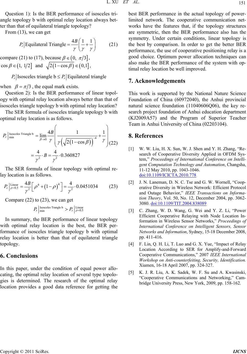

L. XU ET AL.
151
Question 1): Is the BER performance of isosceles tri-
angle topology b with optimal relay location always bet-
ter than that of equilateral triangle topo logy?
From (13), we can get
411
Equilateral Triangle
s
B
P








(21)
compare (21) to (17), because


0, 3  ,


cos1 , 12   and


21 cos0,1  ,
Isosceles triang le bEquilateral tri angle
ss
PP
when 3

 , the equal mark exists.
Question 2): Is the BER performance of linear topol-
ogy with optimal relay location always better than that o f
isosceles triangle topology b with optimal relay location?
The SER formula of isosceles triangle topology b with
optimal relay location is as follows.


Isosceles Triangle b
min 4
0
22
41
lim 21 cos
44
0.360827
s
B
P
B

1

















(22)
The SER formula of linear topology with optimal re-
lay location is as follows.

4
Linear 4
0.5 22
44
1 0.0451034
s
B
P





 (23)
Compare (22) to (23), we can get
Isosceles Trangle bLinear
0.5
min
ss
PP
 

In summary, the BER performance of linear topology
with optimal relay location is the best, the BER per-
formance of isosceles triangle topology b with optimal
relay location is better than that of equilateral triangle
topology.
6. Conclusions
In this paper, under the condition of equal power allo-
cating, the optimal relay location of several type topolo-
gies is determined. The research of the optimal relay
location provides a good data reference for getting the
best BER performance in the actual topology of power-
limited network. The cooperative communication net-
works have the features that, if the topology structures
are symmetric, then the BER performance also has the
symmetry. Under certain conditions, linear topology is
the best by comparison. In order to get the better BER
performance, the use of cooperative position ing relay is a
good choice. Optimum power allocation techniques can
also make the BER performance of the system with op-
timal relay location be well improved.
7. Acknowledgements
This work is supported by the National Nature Science
Foundation of China (60972040), the Anhui provincial
natural science foundation (11040606Q06), the key re-
search project foundation of Anhui education department
(KJ2009A57) and the Program of Superior Teacher
Team in Anhui University of China (022 03104).
8. References
[1] W. W. Liu, H. X. Sun, W. J. Shen and Y. H. Zhang, “Re-
search of Cooperative Diversity Applied in OFDM Sys-
tem,” Proceedings of International Conference on Intelli-
gent Computation Technology and Automation, Changsha,
11-12 May 2010, pp. 1043-1046.
doi:10.1109/ICICTA.2010.778
[2] J. N. Laneman, D. N. C. Tse and G. W. Wornell, “Coop-
erative Diversity in Wireless Network: Efficient Protocol
and Outage Behavior,” IEEE Transactions on Informa-
tion Theory, Vol. 50, No. 12, December 2004, pp. 3062-
3080. doi:10.1109/TIT.2004.838089
[3] C. Zhang, W. D. Wang, G. Wei and Y. Z. Li, “Power
Efficient Cooperative Relaying with Node Location In-
formation in Wireless Sensor Networks,” Proceedings of
International Conference on Intelligent Sensors, Sensor
Networks and Information, Sydney, 15-18 Decemb er 2008,
pp. 411-416.
[4] F. Lin, Q. H. Li, T. Luo and G. X. Yue, “Impact of Relay
Location According to SER for Amplify-and-Forward
Cooperative Communications,” 2007 IEEE International
Workshop on Anti-counterfeiting, Security, Identification.
Xiamen, 16-18 April 2007, pp. 324-327.
[5] K. J. R. Liu, A. K. Sadek, W. F. Su and A. Kwasinski,
“Cooperative Communications and Networking,” Cam-
bridge University Press, New York, 2009, pp. 158-162.