Open Journal of Business and Management, 2014, 2, 65-72
Published Online Janu ary 2014 (http://www.scirp.org/journal/ojbm)
http://dx.doi.org/10.4236/ojbm.2014.21009
Management Analysis of Industrial Production Los ses by
the Design of Experiments, Statistical Process Control, and
Capability Indices
Djida Bounazef1,2, Smain Chabani1, Abdelhafid Idir1, Mokhtar Bounazef3
1HEC, Commercial Graduate School of Algiers, Algiers, Algeria
2Abderrahmane Mira U niversity of Bejaia, Bejaia, Algeria
3Djillali Liabes University of Sidi Bel Abbes, Sidi Bel Abbes, Algeria
Email: dji da.boun azef@ymail.com, incsmachab@gmail.com, a_idir@yahoo.com, Bounazef@yah oo.com
Received November 21, 2013; revised December 23, 2013; accepted J anuary 10, 20 14
Copyright © 2014 Dj ida Bounazef et al. Thi s is an open access art icle distrib uted under the C reative Commons Attrib ution Licen se,
which permits unrestricted use, distribution, and reproduction in any medium, provided the original work is properly cited. In accor-
dance o f the Creative Commons Attribution License all Copyrights © 2014 are reserved for SCIRP and the owner of th e intellectual
property Djida Bo unazef et al . All Copyright © 2014 are guarded by law and by SCIRP as a guardian.
ABSTRACT
The machine stops caused by various breakdowns, rupture of raw materials, production changes, scheduled
maintenance and stops related to human resources management generate an important production loss in the
company. Our ca se study is done in a company t hat manufact ures polyethylene pipes with eig ht production lines.
They stop frequently because they undergo external control factors and noise factors. The method of experi-
mental design that relies on statistical surveys is applied to production loss allows us to observe the action of each
factor on the loss of productio n and t heir int era cti ons of these fa ct ors c ombined in pa irs o n this pro cess. Analy sis
of results shows the dominance of controllable or uncontrollable factor on the loss of production. This is illus-
trated by response surfaces and ISO responses lines were derived by mathematical modelling. Solutions are
proposed to improve continuous production, reduce waste and scrap and therefore increase profitability of
company.
KEYWORDS
Design of Experiments; Production Losse s; Response Surfaces; Polynomial Modelling;
Integrated Management System
1. Introduction
The reduction of industrial wa ste is the major preoccupa-
tion of an integrated management system [1,2] which
includes the environmental management system [3], the
system of qualit y management [4,5] and the manage ment
system of health, security and work [6,7]. These sys-
tems are applied within the company following the re-
quirements of ISO 9001:2000 code 4, until 8.5.3, of ISO
14001:2004 and OHSAS 18001:2007 to achieve optimal
production by minimising work stops caused by various
technical and operational reasons. This integrated mana-
geme nt s ystem [8 -10] is ap plied to the production lines at
the be gi n nin g when checkin g the quality of raw materials
until the end when stor ing fini shed pr od ucts to contribute
in reducing production losses and obtaining finished
quality products. For this, the checks are carried out to
the quality of raw materials, during the production proc-
ess, for finished products and after handling and storage.
Howeve r, the implementation of integrated management
system is not sufficient i n itself, in parallel it is necessar y
to reduce production stops caused by mechanical and
electrical problems, by human resour ce s ma na ge me nt , by
the supplies disruption of raw materials and others. To
know the influence of each breakdown reason of ma-
chinery at each production line, a data record has been
established for a period of one year. These causes were
grouped into 3 categories that encompass these machine
stops into the same types. These categories are the acci-
dental stops, the downtimes due to machine maintenance
and human resource management and the third is stops
due to raw material and finished products. The stops are
OPEN ACCESS OJBM
D. BOUNAZEF ET AL.
66
estimated in work ho urs whereas the loss of production is
calculated as a percentage relative to maximum produc-
tion. The three factors of production stops act simulta-
neously on the loss of production. The application of the
met hod of design of experiments shows how each factor
acts on the loss of production by a mathematical model-
ling and therefore what measures should be taken to
avoid this phenomenon.
2. Statistical Reports of the Causes of
Production Stops
Modelling by design of experiments method analyses the
continuous production process of polyethylene pipes by
measuring ca uses of production losses (waste) caused b y
the steering factors and noise factors. The causes of ma-
chines downtimes that increase the percentage of produc-
tion loses (inducing the waste) are defined by three pa-
rameters on the Ishikawa diagram (Figure 1).
The production process is composed of eight inde-
pendent production lines; their stops are caused sepa-
rately by the same reasons and therefore act on produc-
tion losses (lack of production).
Table 1 shows the distribution of hours of production
losses by types and pr o d uction lines. The accidental stops
are designed by X1, the scheduled stops are designed by
X2 and the stops due to raw material and finished prod-
ucts are designed by X3. Table 1 is called mat rix of ex-
peri men ts, it contains column 6 that means losses of
production expressed in percent. They designate the re-
sponses Y. We see that the line E records the hi gh num-
bers of hours of accidental stops with 2731.83 hours and
human resources management stops with 1085.67 hours,
but it is the line H that has the high number of Stops due
to raw material and finished products with 9703.75 hours.
The greatest loss of production is recorded on line E with
66.18% compared to optimal production. T his is the line
that stores the mos t breakdowns and stops. However, it is
the line C that has the smallest losses of production with
20%.
3. Phenomenon Analysis of Machines Stops
by Design of Experiments Method
The loss of industrial production caused mainly by dif-
ferent stops responds to a mathematical law in polyno-
mial form. This polynomial is a sum of monomials that
are composed of coefficient ai (called parameter effect)
multiplied b y the value of the parameter designated b y xi.
In our study, x1 is letter that represents accidental stops,
x2 is letter that represents maintenance and human re-
sources management stops, and x3 repre sents sto p s due t o
raw material and finished products. In the polynomial,
there are monomials that designate the interactio ns be-
tween the parameters that influence the result; these pa-
rameters are appointed by xixj and
2
ii
x
(i,j=1,2,3); they
must be multiplied b y the valu e of the effect aij. This sum
of these monomials represents the response yi.e. the
loss of production:
011223312 1 213 1 3
222
23 2 311122 2333
ya axax axaxx axx
axxaxaxax
=+++ ++
+ +++
(1)
In the expression 1, the parameters values are coded
values. Generally they are coded because their units and
their scales tha t affect the response y” are different. For
each parameter, we denote by (1) the minimum value,
and by (+1) the maximum value; the intermedia te values
are calculated by the following formula:
min max
max min
2
2
i
i
uu
u
xuu
+



=



(2)
where: Umin is minimal value of parameter, Umax: is
maximal value of parameter, Ui is value to be encoded,
and xi is coded value. Table 2 shows these coded values.
The matrices calculation allows us to ob tain the effects
values ai of parameters b y forming 10 diffe rent equa ti ons
from equat ion 1 by replacing the xi parameters by va lues
from Table 1, we could obtain the 10 coef ficients ai,j by
the followin g formula:
( )
1
tt
a XX XY
=
(3)
Substitutin g the values of ai,j into Equation (1), the
production losses caused by three types of stops is mod-
elled by the following expression:
12 3
1213 23
222
123
37.8259 6.819691.903992.03238
1.30382 8.78769 2.8691
1.422862.72951 0.44013
yxx x
xxxx xx
xxx
=+++
+−−
−++
(4)
4. Results Interpretation
The interpretation is subdivided in two essential parts,
the first consists to analyse causes of production stops of
8 lines of production using design of experiments method,
while the second consists to analyse waste generated by
frequency of production stops using statistical process
control.
5. Analysis of Production Stops Effects by
Experiments Design Method
Equation (4) allows us not only to find the real loss val-
ues of production y” listed in Table 2, but other values
included b et ween the maximum and minimum losses.
This is a predictive and descriptive model. T his is shown
by the estimators of adjusted descriptive quality
2
adjust
R
and predictive quality Q2 of model. Both
2
adjust
R
and Q2
OPEN ACCESS OJBM
D. BOUNAZEF ET AL.
67
Figure 1 . Stops due to raw material and finished pro ducts .
Table 1. Hours of production l osses per line.
Li nes Accidental stops
[H] (X1)
Maintenance and human
resources management stops
[H] (X2)
Stops due to raw material and
fin ished pr oduc ts
[H] (X3)
Produ ction losses
[%] (Y)
1 Li ne A 220.8 798.92 988.08 2 2.49
2 Line B 1692.8 844.08 1048 40
3 Line C 153.67 815.75 795.08 20
4 Li ne D 1891.75 669.42 1291.83 43.27
5 Li ne E 2731.83 1085.67 2074.75 66.18
6 Line F 1393.5 876.92 1515.58 42.52
7 Li ne G 741.88 859.67 779.17 26.74
8 Li ne H 1690.33 795.61 9703.75 41.26
Table 2. Coded values of several st ops of machines.
Li nes Coded accidental stops
(X1)
Coded maintenance and human
resources management stops
(X2)
Coded values of stops due to raw
material and finished products
(X3)
Produ ction losses
(Y)
1
Li ne A
0.9479241
0.37777778
0.95318323
0.89216111
2 Li ne B 0.19397555 0.16079279 0.93975515 0.13382417
3 Li ne C 1 0.29691291 0.99643457 1
4 Line D 0.34831042 1 0.8851128 0.00779558
5 Line E +1 +1 0.70 966029 +1
6 Li ne F 0.03820554 0.003003 0.83497039 0.02468601
7 Li ne G 0.54369783 0.08588589 1 0.70809874
8 Line H 0.19205945 0.39368168 +1 0.07925509
values are numbers usually between ‒∞ and 1. Values
close to 1 for both
2
adjust
R
and Q2 indicate very good
model with excellent predictive result. In our case
2
adjust
0.903R=
and Q2 = 0.863. The first estimator re-
flects the co ntribution of the model in the restitution of
the observed response and the second estimated coeffi-
cient reflects the ability of the model to predict res ponse
without making statistical measurements or experiments.
To illustrate these results, the Figure 2 shows the devia-
tions of measurement points relative to b isec tor.
The details of deviations are shown in Table 3 where
one see s tha t the maximu m deviatio n is estimat ed to 7.9%
in measurement 7. The Student test shows us if the vari-
able xi or the interaction xi,j associated with ai,j affects
response “yor not. For this, one calculates the coeffi-
cient ti of Student as follo ws:
i
ii
a
ts
=
(5)
With
2
i
s
is variance of effects; it is calculated by fol-
lowing :
2
2
i
s
sn
=
(6)
where s2 is estimator of polynomial effects; it is calcu-
lates by this formula:
22
1
i
se
np
=
(7)
Here, n is equations number ob tained b y combinations
of values of xi,j from Table 1, it is equal to 33 = 27 (full
factorial design), and p is number of modelling coeffi-
OPEN ACCESS OJBM
D. BOUNAZEF ET AL.
68
20
30
40
50
60
20 30 40 50 60
Observed
Predicted
1
2
3
4
5
6
7
8
Figure 2 . O bserv ed vs. Predicted plot.
Table 3. Deviations between predic ted and observed values.
Observed Predicted Difference
1 22.49 21.6865 0.803453
2 40 41.2669 1.26685
3 20 19.7343 0.265732
4 43.27 43.4725 0.202545
5 66.18 66.331 0.151001
6 42.52 39.1532 3.36685
7 26.74 29.5363 2.79629
8 41.26 41.2793 0.0193405
cients, it is equal to 10 (see Equation (1)). The compari-
son between tcrit taken from Student table for risk α =
0.05 and freedom degree ν = 17, shows that all “ti” are
higher than tcrit = 0.689, it means that all variables xi,j
influence the responsey”, i.e. the loss of production
(Table 4).
Equation (4) allo ws working simultaneously the three
parameters in the field of work but we cannot interpret it
graphically. However, we vary two parameters while
leaving unchanged the third par ameter (x3).
6. Production Losses According Accidental
Stops When x2 and x3 Are Middle Values
To observe how the losses of production vary according
one parameter, one gi ves to 2 others parameters in Equa-
tion (4) permanent middle values. We can then plot the
variation of production losses according one of 3 pa-
rameters. The statistics collected during the production
indicate that while stabilising the production losses due
to raw materials and finished products as well as main-
tenance to their middle values (x2 = 877.7 hours, x3 =
5241.6 hours), one reaches the maxi mum val ue of 40.5%
of production losses at 900 hours of accidental stops. The
mathematical modelling decreases these losses to 34.3%
at 2730 hours (Figure 3). When x1 exceeds the value of
900 hours, x2 and x3 are statisticall y acting on the model
and are decr easing production losses.
Table 4. Student coefficients.
2
21.5401757
i
e=
; s2 = 1.26706916
20.04692849
i
s=
; si = 0.21662984
t1 174.61 t6 40. 56
t2 31.48 t7 13.24
t3 8.79 t8 6.57
t4 9.38 t9 12.60
t5 6.02 t10 2.03
Figure 3. Graph of production losses acco rding accidental
stops.
7. Production Losses According
Maintenance and Human Resources
Management Stops When x1 and x3 Are
Middle Values
Maintaining accidental stops x1 and stops due to ra w ma-
terial and finished products x3 constant respectively at
1476.40 hours and 5241.6 hours, o ne varies only x2 from
its minimum value to its maximum value, we obtain a
minimal loss of production of 39.8% for x2 = 860 hours
(Figure 4).
This means that the parameter x2 has a positive influ-
ence in reducing production losses in the model (4), but
from x2 = 860 hours, fact ors x1 and x3 are more influential
than x2. This explains why the curve increases until pro-
duction losses of 50.2% for x2 = 1090 hours.
OPEN ACCESS OJBM
D. BOUNAZEF ET AL.
69
Figure 4. Graph of production losses according mainte-
nance and human resources manag ement st ops.
8. Production Losses According Stops Due to
Raw Material and Finished Products
When x1 and x2 Are Middle Values
When we leave constant x1 = 1476.40 hours and x2 =
877.70 hour s (middle values), we note that the minimum
losses of production is q uickly rea ched at 30.8% for x3 =
3260 hours when the curve decreases. This shows that
from this minimum, the factors x1 and x2 are increasing
the response “y” (production losses) when x3 varies from
its minimum value to maximum value (Figure 5).
9. Results Interpretation When x1 and x2
Are Varied Together
For this, one gives to third parameter x3 an invariable
value and one changes the 2 other from their minimum
value to their maximum value. One can plot response
surfaces in three dimensions and c urves iso -responses in
two dimensions to illustrate the action of two parameters
simultaneously on the production losses.
10. When x3 Is Equal at the Low Value
(x3 = 779.17 Hours)
In this case, the response surface is concave rectangular
form; it shows parallel areas of production losses ma i n ly
when accidental stops (x1) and stops caused by ma i nt e-
nance and management of human resource s (x2) are high
(Figure 6).
When accidental stops are less than 1500 hours, these
areas are parallel to the axis of x2. It shows that acciden-
tal stops act very low in the model response. All this is
visible on curves ISO response, where one notes that the
losses of production remains relatively constant between
20.8% and 24.2% for stops due to maintenance and
management of human resources between 675 hours and
937.5 hours. From 1330 hours of accidental stops that the
increase of x2 increases clearly the production losses.
11. When x3 Is Equal at the Middle Value
(x3 = 5241.60 Hours)
When x3 takes the mid dle val ue of 5241.6 hours, the ma -
Figure 5. Graph of production losses according stops due
raw material and finished pr oduc ts.
Figure 6. Response surface and ISO response curves when
x3 is low.
thematical model (4) presents respo nse s surface as a sad-
dle of horse (Figure 7). Its complexity shows how the
simultaneous influence of x1 and x2 acts on production
los ses of finished products. The projection of the re-
sponse surface on the lower plane gives ISO responses
curves that’s the central part is in the form of four ten-
OPEN ACCESS OJBM
D. BOUNAZEF ET AL.
70
Figure 7. Response surface and ISO response curves when
x3 is middle.
tacles. In t his section, the resp onse yremains relativel y
constant; it varies from 40.5% to 41.3% over a large part
of the work domain. T his shows tha t we can get the con-
stant value of production losses defined by the 41.3% by
several combinations between accidental stops (x1) and
maintenance and manage ment of human resources stops.
Table 5 gives some values of production losses outside
the central zone with tentacles.
It is clear, that the columns and rows (Table 5) display
for constant values of the parameter x1, that production
losses decrease in first with increasing parameter x2, sta-
bilise at central area of the graph 8, and subsequently
increase. However, when x2 re mains c onsta nt, production
losses decrease for the 2 first rows with increasin g x1, but
increase in first and subsequently decrease for the 2 last
r ows of Table 5 with increasing x1.
12. When x3 Is Equal at the High Value
(x3 = 9703.75 Hours)
When the parameter x3 take s i ts ma ximu m a nd invariable
Table 5. Pr oduction loss e s in cent r a l zone when x3 is middle.
x1
x2 500
hours 1000
hours 1500
hours 2000
hours 2500
hours
700
hours 47.4% 46.5% 44.7% 42% 38.4%
750
hours 44.1% 43.5% 42% 39.7% 36.4%
1000
hours 42.7% 43.8% 43.9% 43.1% 41.4%
1050
hours 45.5% 46.9% 47.3% 46.8% 45.4%
value of 9703.75 hours in the mathematical model 4, the
responses surface is the concave form upwards (Figure 8).
Its projection gives curves ISO responses directed from
top to bottom and curved in the centre of the graph. This
shows that for a given value of accidental stops (x1),
losses of production vary slowly with the c ha n ge of stops
due to maintenance and human resource management. It
is easy to see that for maximum value of x3 = 9703.75
hours, the increase of accidental stops (x1) reduced the
losses of production; this is due to the effect of negative
sign of the interaction of parameters x1 and x3 in the
polynomial (4) and equal to a13 = 8.78769 which re-
duces considerably the value of the response “y”. One
remarks that in passing from value x1 = 500 hours to
x1=2500 hours for the same value of x2 = 900 hours,
losses of production fells from 55.8% to 22.2 %.
13. Management of Production Waste by
Statistical Process Control
The losses rate of production per lines caused by the
various stops does not explain alone the waste of fini s hed
products during production process. It is r at her frequency
of repeated stops that causes restarts manufacturing
process. T his will requires each time the equipments set-
tings to obtain the finished standardised products. Know-
ing annual waste rate of polyethylene products for water
of 3.15% and for ga s of 2.54%, the average waste rate of
8 lines is:
1
Waste rate2.845%
n
i
i
x
n
=
= =
(8)
where:
i
x
is sum of distribution values equal to
5.69%; n is samples number equal to 2; this is giving us
process quality “m” or “Yield” of 97.155% (Figure 9).
This value is considered as the average value of the
process target to achieve (average value of distribution).
As the value of the standard deviation is sigma equal to
0.9425071, the repetition frequency of production stops is:
10.42328
2π
f
σ
= =
(9)
OPEN ACCESS OJBM
D. BOUNAZEF ET AL.
71
Figure 8. Response surface and ISO response curves when
x3 is high.
Thi s val ue i s represented by the top of the Gauss c ur v e
of production process. It corresponds to 0.91569σ on the
X axis and represents the lag due to the production proc-
ess and waste estimated at 28500 DPMO (defects per
millions of opportunities) (U n hatched area of Figure 9).
The beginning of waste area corresponding to end of
process performance z, it is found in the following man-
ner:
coefz
σ
= ⋅
(10)
where z is sigma process quality; it is calculated with
coefficient who take n from the normal distrib ution taking
acco unt the risk of 0.05 and “UCL, LCL” values through
manufactured tables (coef = 3.403311); the process per-
formance z is equal at 3.403311σ. The σ value is the
standard de viation, it calculated by this formula:
()
2
1
n
i
xm
n
σ
=
(11)
Figure 9 . Gauss curve of pro duction lo s ses .
The process performance z is then 3 .20 76447. The lo w
control limit (LCL) and the upper c ontrol limit (UCL) ar e
calculated by this following formula; here, the target is
the process quality m = 100% ‒ 2.845% = 97.155%:
LCL,UCLtarget 3
σ
= ±
(12)
Their respective values are then 94.327419 and
100.377521. The process quality area of the real produc-
tion process is thus defined by LCL, UCL and the Gauss
curve of normal distribution (hatched zone in Figure 9).
It is equal to 97.155%. The combination of two methods
of analysis, the experimental design and statistical proc-
ess control in management showed us that performance
of studied process is relatively small compared to a
process without stops or waste. The management of
waste during the production process is directly linked to
the frequency of stops and starts of manufacturing lines.
To achieve Six Sigma pr ocess with performance of
99.999%, one must impr ove the process capability index
Cp in order to be higher than 2. However, the capability
index of six production lines is z/3 = 1.1344; the produc-
tion process of PE is then just capable. To achieve high
performance, one must act in several fields that cause the
increase of waste. Managing production waste is to un-
der stand the real causes that pus h businessmen to s ubmit
pro gra m change s on the production lines, and see if there
are opportunities for t heir red uctions. It must also under-
stand the real causes o f mechanical and electrical failures
and assess the reliability of the maintenance planning.
Finally know the real causes of non conformities of
products and analyse the production process and inter-
vention function responsible for the technical quality.
Thereafter take the necessary technical and financial
measures and control by means of managerial actions to
reduce this waste.
14. Capability Indices and Process
Performance
The capability indices of process “Cp”, of machine “Cm
and process performance “Pp” are important data that de-
monstrate the real capacity continuous production pro-
OPEN ACCESS OJBM
D. BOUNAZEF ET AL.
72
cess of the manufacturing company of tubes. The capa-
bility index that takes account process, machine, and the
performance is calculated as follows:
( )
UCL LCL
Index, ,6
pmp
CCP
σ
=
(13)
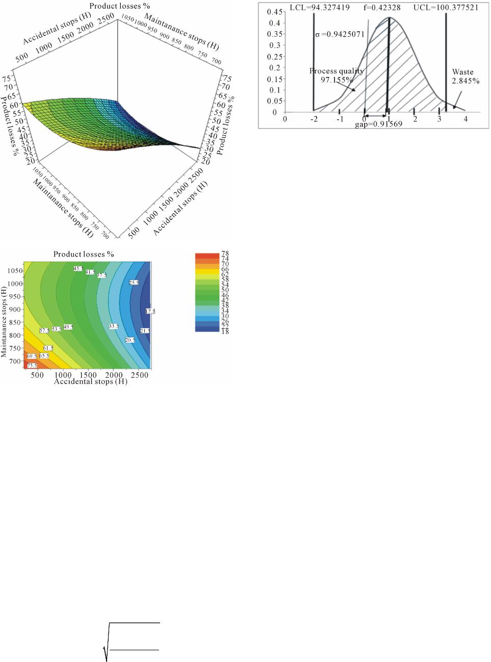
The val ue of t hi s i nd e x i s t he n 0 , 9 999 9 3 , i. e . close to 1.
The capability index of the process Cp is found in the
following manner:
3.2076447 1.0692149
33
p
z
C= ==
(14)
The Cp index exceeds the value of 1, but the quality of
process 6σ requires a capability of process more than 2.
The production process of the tubes is barely capable but
is not very efficient. The capability index of Machine Cm
allows measuring the material resources available the
continuous production process of the tubes is able to
achieve the target of 99.999966% of performance; the
value of this ind e x is :
( )
2
1
UCLLCL;
3
target
;
1
0.6292
m
n
i
i
m
C
x
n
C
σ
σ
=
=
=
=
(15)
The Cm index does not exceed 1.11 which allows the
reduction of waste of 0.00034%. The tools and machin-
eries of production plant are not capable to achieve per-
formance of 6σ quality. The plant must innovate and re-
duce the variability due to different causes of machine
stops.
15. Conclusion
Causes a nalysis of wa ste by 2 methods statistica l process
control and design of experiments are a very effective
means that can take me asures to manage the losses.
These methods permit to develop recommendations.
They can satisfy demands to achieve the production re-
quirements mastering the c ontrollab le factors, reducing
the impact of uncontrollable factors, minimising the fi-
nancial losses and improving the quality of production.
The reduction of waste is the result of the reduction of
machine stops; this reduction supports the achievement
of measurable and non-measurable gains such as reduc-
tion of the manufacturing cost and coast of control fac-
tors, reduction delay time, improvement employee com-
petence, improvement working environment due to the
reduction of machine stops hours. All this will automati-
cally change the pr ofitability of the process and the gains
of the company. The performance of production is treat-
ed in sigma process quality (performance quality) by
Equation (10).
REFERENCES
[1] P. Bousselet, “The process Computerisation QSE in Ag-
ribusiness: The 30 Questions to Consider Quality, Safety
and Environment,” PBC Soft, Paris, 2010.
[2] B. F r o ma n, J. M. Gey and F. Bonnifet, “Quality, Safety
and Environment: Construct an Integrated Management
Sys te m, ” AFNOR, La Plaine Saint-Denis, 2007.
[3] M. Bernardo, M. Casadesus and S. Karapetr ovic, “How
Integrated Are Environmental, Quality and Other Stan-
dardised Management Systems? An Empirical Study,”
Journal of Cleaner Production, Vol. 17, No. 8, 2009, pp.
742-750. http://dx.doi.org/10.1016/j.jclepro.2008.11.003
[4] K. R. Bhote, The Po wer of Ultimate Six Sigma, Quality
Excellence t o To tal B usi ness E xc el len ce,” Amacom, New
York, 2003.
[5] D. Duret and M. Pillet, “Quality in Production: From ISO
9000 to Six Sigma,4th Edition, Eyrolles Edition, Paris,
2005.
[6] H. Aadi and B. John, Hygiene and Safety at Work,
Office of Professional Training and Work Promotion,
Rabat, 2011.
[7] Fernand ez-Toro and A. H. Schauer, “Management of
Information Security: Implementing ISO 27001, Imple-
mentation of ISMS and Certification Audit,” Eyrolles,
Paris, 2008.
[8] R. Holdsworth, “Practical Applications Approach to De-
sign, Development and Implementation of an Integrated
Management System,” Journal of Hazardous Materials,
Vol. 104, No. 1-3, 2003, pp. 193-205.
http://dx.doi.org/10.1016/j.jhazmat.2003.08.001
[9] T. H. Jorgensen, A. Remmen and M. D. Mellado, “Inte-
grated Management Syste ms Three Levels of Integra-
tion,” Journal of Cleaner Production, Vol. 14, 2006, pp.
713-722.
[10] R. Salomone, “Integrated Management S ys t em s : Experi-
ences in Italian Organisations,Journal of Clearner Pro-
duction, Vol. 16, 2008, pp. 1786-1805.
OPEN ACCESS OJBM