Psychology
2014. Vol.5, No.1, 6-11
Published Online January 2014 in SciRes (http://www.scirp .org/journal/psych) http://dx.doi.org/10.4236/psych.2014.51002
Efficiency of Selecting Important Varia ble for Longitudinal Data
Jo ngmi n Ra, Ki-Jong Rhee
Department of Educa tion, Kookmin University, Seoul, Sout h Korea
Received O ctober 12th, 2013; revised November 13th, 2013; accept ed Decem ber 9th, 2013
Copyright © 2014 Jongmin Ra, Ki-Jong Rhee. This is an open access article distributed under the Creative
Commons Attribution License, which permits unrestricted use, distribution, and reproduction in any medium,
provided the original work is properly cited. In accordance of the Creative Commons Attribution License all
Copyrights © 2014 are reserved for SCIRP and the owner of the intellectual property Jongmin Ra, Ki-Jon g Rhee.
All Copyright © 2014 are guarded by law and by SCIRP as a guardian.
Varia ble selec tion wi th a large nu mber of pr edictors is a very cha llenging a nd impor tant prob lem in edu-
cati onal and s ocial doma ins. Howe ver, rel ativel y littl e attent ion has b een paid t o issues of vari able sel ec-
tion in longitudinal data with application to education. Using this longitudinal educational data (Test of
English for International Communication, TOEIC), this study compares multiple regression, backward
elimination, group least selection absolute shrinkage and selection operator (LASSO), and linear mixed
models i n terms of t heir p erformance i n variabl e selection. The resul ts from the s tudy show tha t four di f-
ferent statistical methods contain different sets of predictors in their models. The linear mixed model
(LMM) provides the s mallest number of predi ctors (4 predic tors a mong a tota l of 19 pr edic tors). In a ddi-
tion, LMM is the onl y ap propria te method for the r epeated mea surement a nd is the bes t method with re-
spect to t he pri ncipa l of pa rsi mony. This s t udy als o provides int er p reta tion of the sel ec ted model b y LMM
in the conclus ion using marginal
2
R
.
Key words: Group LASSO; Li near Mi xed M odel; Longitudinal D ata; Marginal
2
R
; Variable Selection
Introduction
The characteristic of a longitudinal study is that individuals
are measured repeatedly through different time points and re-
quir e special statisti cal methods because th e set of observatio ns
on the same individual tends to be inter-correlated and can be
explained by both fixed and random effects.
As longitudinal data are common in educational settings, the
linear mixed model (LMM) has emerged as an effective ap-
proach since it can model within and between subject hetero-
geneity (Vonesh, Chinchilli, & Pu, 1996). The LMM also at-
tempts to account for within-subject dependency in the multiple
measurements by including one or more subject-specific vari-
ables in a regression model (Laird & Ware, 19 82; Giks, Wang,
Yvonnet, & Coursaget, 1993).
Despite the development of statistical models, model selec-
tion criteria for the LMM h ave received little attention (Orelien
& Edwards, 2008; Vonesh et al., 1996). However, several stud-
ies (Vonesh & Chinchilli, 1997; Vonesh et al., 1996; Zheng,
2000) recently suggest model fit indices which are useful for
mixed effect models. More specifically, studies (Vonesh &
Chinchilli, 1997; Vonesh et al., 1996) show that marginal
2
R
is preferred when only fixed-effect components are involved in
the predicted values, but conditional
2
R
is preferred for ran-
dom effects (Vonesh et al., 1996).
It is not uncommon to collect a large number of predictors to
model an individual’s reading achievement more accurately in
educational and psychological fields. Thus, it is fundamental to
select meaningful variables in multivariate statistical models
(Zhang, Wahba, Lin, Voelker, Ferris, Klein, & Klein, 2004) to
increase prediction accuracy and to provide better understand-
ing of concepts.
It is, however, ch allen gin g to select impor tan t variabl es when
a respon se vari abl e is measured rep eated ly over a cert ain per io d
of time because it is known that the selection process of statis-
tically significant variables is hindered by the correlation
among th e repeated measure ment s. Furthermore, classical vari-
able selection methods, such as the forward selection and the
backward elimination methods are time-consuming, unstable,
and sometimes unreliable for making inferences. Although
there is a great deal of e xtent rese arch examin in g issu es o f var i-
able select ion in linear regressi on, little research has been don e
investigating how differently and similarly different statistical
methods perform within a longitudinal data. This study aims to
investigate how similarly and differently various statistical
method s perform in the presen ce of the rep eated mea surements
in the d ata.
Hence, thi s study compares fo ur different statist ical method s,
multiple regression, backward elimination, group least selection
absolute shrinkage and selection operator (LASSO), and the
LMM, using a test of English as International Communication
(TOEIC) data as individuals’ reading achievement. For the
LMM, marginal
2
R
for remaining variables in the model is
used to provide a better understanding of the impacts of se-
lected predictors in the longitudinal data.
Multiple Linear Regression
Mult iple linear r egression is a flexible method o f data anal y-
sis that may be appropriate whenever a response variable is to
be examined in relation to any other predictors (Cohen, Cohen,
OPEN ACCE SS 6

J. RA, K.-J. RHEE
West, & Aiken, 2003). For instance, if a multiple regression
method is used for predicting and explaining an individual’s
English achievement, many variables such as gender, age, and
socio -economic status (SES) might all contribute toward indi-
vidual’s En glish achievement.
The multiple regression method for predicting English achieve-
ment, Y, with the observed data
( )
1, ,,1,, , i pi
X Xin=
is as
follows
0112 2iiip pii
Y XXX ββ ββε = +++++
. This equation
shows the relationship between p predictors and a response
variable Y, all of which are measured simultaneously on the
subject. This method is called linear because the effects of the
various pred ictors are treated as addit ive.
In addition, much efforts has been put to estimate the per-
formance of different methods and choose the best one by using
fit indices such as AIC (Akaike, 1973), BIC (Schwarz, 1978),
Mellow’s
p
C
(Mallows, 1973), and adjusted
2
R
. AIC and
BIC are bas ed on th e penalized maximum likelih ood estimat es.
AIC is defined as −2log(L) + 2p, where log(L) is the loglikeli-
hood function of the parameters in the model evaluated at the
maximum likelihood estimator while the second term is a pen-
alty term for additional parameters in the model. Therefore, as
the number of independent variables included in the model
increases, the first term decreases while the penalty term in-
creases. Conversely, as variables are dropped from the model,
the lack of fit term increases while the penalty term decreases.
BIC is defined as
()( )
2log logLp n− +×
. The penalt y term for
BIC is similar to AIC but uses a multiplier of log(n) instead of a
constant 2 by incorporating the sample size. In general, AIC
tends to choose overly complex models when sample size is
large and BIC tends to choose overly simple model when sam-
ple size is small and also choose the correct model when sam-
ple size approaches infinity.
Mallow’s
p
C
is als o co m mo nl y u sed to i n v es ti g at e how we l l a
mod el fits d ata and can b e defin ed as
2
2()
pp
C SSEpn σ += +

.
In this equation,
ˆ
σ
represents the estimate of
2
σ
and
p
SSE
is defined as
( )
2
11
ˆ
np
i ii
ii
YX β
= =
−
∑∑
, where
ˆ
β
is the estimator
of
β
. Mallow’s
p
C
is calculated for all possible subset
models. The model with the smallest value of
p
C
is deemed
to be the best linear model. As the number of independent
variables (p) increases, an increased penalty term 2p is offset
with a decreased SSE.
Another commonly used fit index for model selection is
2
R
or adjusted
2
R
. Both
2
R
and adjusted
2
R
represent the
percentage of the variability of the response variable that is
explained by the variation of predictors.
2
R
is a function of
the total sum of square (SST) and SSE, and the formula is given
by
( )
1SSE SST−
.
Adjusted
2
R
takes into account the degrees of freedom
used up by adding more predictors. Even though adjusted
2
R
attempts to yield a more robust value to estimate
2
R
, there is
little difference between adjusted
2
R
and
2
R
when a large
number of predictors are included in a model.
When the number of observations is very large compared to
the number of predictors in a model, the value of
2
R
and ad-
justed
2
R
will be much closer because the ratio of
() ()
n1 n1p−−−
will approach 1. Despite the practical ad-
vantages o f using a multiple regression method, it is difficult to
build multiple regression models for repeatedly measured re-
sponses. The multiple regression method is not appropriate for
correlated response variables as in longitudinal data without
accounting for correlation within response variables.
Backward Elimination Approach
Besides the multiple regression approach, backward eli mina-
tion is common and important practice to select relevant vari-
ables among a large number of predictors. A subset selection
method is one of the most widely used variable selection ap-
proaches in which one predictor at a time is added or deleted
based on the F statistic iteratively (Bernstein, 1989). Subset
selection methods, in general, provide an effective means to
screen a large n u mber of var iab les (Ho smer & Lmeshow, 2000).
Since there is a possibility of emerging a suppressor effect in
the forward inclusion method (Agresti & Finlay, 1986), the
backward elimination method is usually preferred method of
exploratory analysis (Agresti, 2002; Hosmer & Lemeshow,
2000; Menard, 1995) and follows three steps.
First, obtains a regression equation which includes allp pre-
dictors. Second, conducts a partial F-test for each of the pre-
dictors which indicates the significance of the corresponding
predictor as if it is the last variable entered into the equation.
Finally, selects the lowest partial F value and compares it with
a threshold partial,
F
α
, the value set equal to some predeter-
mined level of significance,
α
If the smallest partial F is less
than
F
α
, then deletes that variable and repeats the process for
p − 1 predictors. This sequence continues until the smallest
partial
F
α
at any given st ep i s gr eat er th an
F
α
. The variab le s
that are remained in the model are considered as significant
predictors. In general, the backward elimination method is
computationally attractive and can be conducted with an esti-
mation accuracy criterion or through hypothesis testing.
The backward elimination method, however, is far from p er-
fection. This method often leads to locally optimal solutions
rather than globally optimal solution. Also, the backward
elimination method yields confidence intervals for effects and
predicted value that are far too narrow (Altman & Andersen,
1989). The degree of correlation among the predictors affects
the frequency with which authentic predictor find their way into
the final model in terms of frequency o f obtaining authentic and
noise predictors (Derksen & Keselman, 1992). More specifi-
cally, the number of candidate predictors affects the number of
noise predictors that gains entry to the model. Furthermore, it is
well known that the backward elimination method will not
necessarily produce the best model if there are redundant vari-
ables (Derksen & Keselman, 1992). It also yields
2
R
values
that are badly biased upward and have severe problems in the
presence of collinearity. Since the backward elimination me-
thod gives biased re gression coefficient esti mates, they need t o
be shrunk because the regression coefficients for remaining
variables are too large. Besides well-known inherent technical
problems, it is time consuming when a large number of predic-
tors are included in the model and cumbersome to choose ap-
propriate variables manually when categorical variables are
includ ed in the model as a dummy variable.
The Group LASSO
To overcome problems shown in multiple regression and
backward elimination approaches, a number of shrinkage
methods are developed to overcome the inherent problem
shown in traditional variable selection methods (Bondell &
Reich, 2008; Forster & George, 1994; George & McCulloch,
1993; Tibshirani, 1996). Among many suggested shrinkage
methods, the least absolute shrinkage and selection operator
OPEN ACCE SS 7

J. RA, K.-J. RHEE
(LASSO) suggested by Tibshirani (1996) is one of well-known
penalized regression approaches (Bondell & Reich, 2008;
Meier, van de Geer, & Bhlmann, 2008; Tibshirani, 1996). The
LASSO method minimizes the residual sum of squares subject
to the sum of the absolute value of the coefficients being less
than a constant (Tibshirani, 1996). It is also well known that all
the variables in LASSO type methods such as the standardized
LASSO and group LASSO (Yuan & Lin, 2006) need to be
standardized before performing analysis.
The LASSO method is defined as follows
( )
( )
2
0
10 1
ˆ
minarg npp
LASSO ii
ii i
YX
β
β λβλβ
= ==
= −+
∑∑ ∑
In this
equation,
( )
01
,,
p
β βββ =
and
λ
is a penalty or tuning
parameter. The parameter  controls the amount of shrinkage
that is applied to the estimates. The solution paths of LASSO
are piecewis e linear, and thus can be compu ted very efficien tly.
The variables selected by the LASSO method are included in
the model with shrunken coefficients. The salient feature of the
LASSO method is that it sets some coefficients to be 0 and
shrinks others. Furthermore, the LASSO method has two ad-
vantages co mpared to the trad itional estimati on method . One is
that it estimates para meters an d select variables si multaneously
(Tibshirani, 1996; Fan & Li, 2001). The other is that the solu-
tion path of the LASSO method moves in a predictable manner
sine it has good computational properties (Efron, Hastie,
Johnstone, & Tibshirani, 2004). Thus, the LASSO method can
be used for high-dimensional data as long as the number of
predictors, is smaller than or equal ton,
pn
≤
.
The LASSO method, however, has some drawbacks (Yuan
& Lin, 2006). If the number of predictors (p) is larger than the
number of observations (n), the LASSO method at most select
variables due to the nature of the convex optimization problem.
Also, the LASSO method tends to make selection based on the
strength of individual derived input variables rather than the
strength of groups of input variables, often resulting in select-
ing more variables than necessary. Another drawback of using
the LASSO method is that the solution depends on how the
variables are orthonormalized. That is, if any variable
i
X
is
reparameterized through a different set of orthonormal contrasts,
there is a possibility of getting different set of variables in the
solution. This is undesirable since solutions to a variable selec-
tion and estimation problem should not depend on how the
variables are represented. In addition, the LASSO solutions
brin g another problem when cat egorical variab les enter into the
model. The LASSO method treats categorical variables as an
individual variables rather than a group (Meier et al., 2008). A
major stumbling block of the LASSO method is that if there are
groups of highly correlated variables, it tends to arbitrarily se-
lect only one from each group. This makes models difficult to
interpret because p redictor s th at are strongly associated with the
outcome are not included in the predictive model.
To remedy the shortcomings of the LASSO method, Yuan
and Lin (2006) suggested the group LASSO in which an entire
group of predictors may drop out of the model depending on.
The group LASSO is defined as follows
( )
2
11
1 11
minarg Lp
LASSO ll
li
YX P βλλ β
= =

= −+


∑∑
In this
equation,
l
X
represents the predictors corresponding to the
lth group, with corresponding coefficient sub-vector, and
l
β
.
l
P
takes into account for the different group sizes. If
( )
1,T k
xxx=
, then,
2
2
11
k
i
i
x x
=
=
∑
. The group LASSO acts
like the LASSO at the group level; depending
λ
, an entire
group of predictors may drop out of the model. The group
LASSO takes two steps. First, a solution path indexed by cer-
tain tuning parameter is built. Then, the final model is selected
on the solution path by cross validation or using a criterion such
as the Mallow’s
p
C
.
This gives group LASSO tremendous computational advan-
tages when compared with other methods. The group LASSO
makes statistically insignificant variables become zero by in-
corporating shrinkage as the standard LASSO do es . Overall, the
group LASSO method enjoys great computational advantages
and excellent performance, and a number of nonzero coeffi-
cients in the LASSO and the group LASSO methods are an
unbiased estimated of the degree of freedom (Efron et al.,
2004).
Even though the group LASSO is suggested for overcoming
drawbacks for the standard LASSO, the group LASSO method
still has some limitations. For example, the solution path of the
group LASSO is not piecewise linear which precludes the ap-
plication of efficient optimization methods (Efron et al., 2004).
It is also known that the method tends to select a large number
of groups than necessary, and thus includes some noisy vari-
ables in the model (Meier et al., 2008). Furthermore, the group
LASSO method is not directly applicable to longitudinal data
and needs further study for being suitable for the repeated
measurement. R code for the group LASSO is provided in
Appendix.
Linear Mixed Model
The linear mixed model (LMM) is another very useful ap-
proach for longitudinal studies to describe relationship between
a response variable and predictors. The LMM has been called
differently in different fields. In economics, the term “random
coefficient regression models” is common. In sociology, “mul-
tilevel modeling” is common, alluding to the fact that regres-
sion intercepts and slops at the individual level may be treated
as random effects of a higher level. In statistics, the term
“variance components models” is often used in addition to
mixed effect models, alluding to the fact that one may decom-
pose the variance into components attributable to within-groups
versus between-groups effects. All these terms are closely re-
lated, albeit emphasizing different aspects of the LMM. In the
context of repeated measure, let
i
Y
is an
1
i
n×
vector of
observations from the ith subject. Then, the LMM (Laird &
Ware, 1982) is as follows
iiii i
Y XZb βε = ++
.
In this model,
( )
1, ,
T
t
ii pi
X XX=
, where
i
X
is an
i
n p×
fix e d effect design matrix whereas
i
Z
are known
i
nq×
const ant design matr ices.
( )
1
,
T
p
βββ =
is an p-dimensional
vector and unknown coefficients of the fixed effects. Here,
i
b
is assumed to be multivariate normally distributed with mean
vector 0 and variance matrix
Ψ
. Thus, the random effects
vary by group. In addition, variance-covariance matrix
Ψ
=
diag
( )
Ψ,Ψ
should be symmetric and positive semidefinite
(Laird & Ware, 1982). The
i
ε
are vectors of error term and
assu med to follow a normal distribution with mean vector 0 and
variance-covariance matrix ,
Ω
, which are the same for all
subjects. It is also commonl y assumed th at
Ω
is di agonal and
all diagonal values are equal,
2
σ
. However, instead of assum-
ing equal variance in grouped data, it is possible to extend to
allow unequal variance and correlated within-group errors.
The vectors
i
b
and
i
ε
are assumed to be independent.
8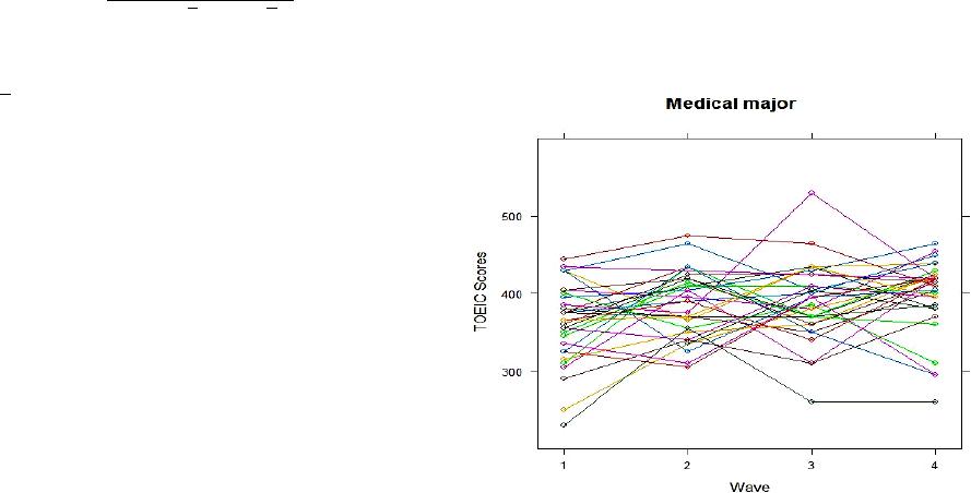

J. RA, K.-J. RHEE
Method
Participants and Va r i ables
This study takes place in a public university in Republic of
Korea, between the years 2009 and 2010, over two semesters.
Participating students (n = 281) enrolled in TOEIC classes for
four hours a week. Except students’ TOEIC scores, Th e TOE I C
dataset records 20 predictors. Among 20 predictors, 13 are
continuous: age, father’s education level (FEL), mother’s edu-
cation level (MEL), SES, English study time (EST), reading
time, level of reading competence (LRC), materials written in
English (ME), level of computer skill (LC), length of private
tutoring (LPT ) , three mean-centered cognitive assessment
scores (STAS: State and trait anxiety scale, FLCAS: Foreign
language classroom anxiety scale, FRAS: Foreign language
readin g anxiety scale); an d 7 are categorical: major, gen der, ex-
perience of private tutoring (EPT), experience of h avi ng foreign
instructors (EFI), living areas, length of staying at abroad
(LSA), experience of staying English speaking countries (ESE).
The wave 2, 3, and 4 data ar e collected ever y t hree mont hs after
collect ing wave 1 dat a.
Procedures
All the analysis are p erformed with R (R Development Core
Team, 2013) due to the unavailability of the group LASSO
approach in standardized statistical packages such as SPSS.
Once statistically significant predictors in the model are ob-
tained, goodness-of-fit for the LMM can be considered. Among
different types of 2such as unweighted concordance correla-
tion coefficient (CCC: Venesh et al., 1996), and proportional
reduction in penalized quasi-likelihood (Zheng, 2000), the mar-
ginal
2
R
(Vonesh & Chinchilli, 1997) is easy to compute and
interpret in that it is a straightforward extension of the tradi-
tional
2
R
(Orelien & Edwards, 2008). The marginal
2
R
in this
analysis for s electin g relevant vari ables is defined as follo ws
() ()
() ( )
1
2
1
ˆ ˆ
1
T
n
ii i
i
mT
n
i pii pi
i
YY YY
RYY YY
=
=
−−
= −−−
∑
∑
.
Given the equation shown above,
,nof observations, is a
observed response variable and
ˆi
Y
is a predicted response
variables.
i
Y
is the grand mean and is an vector of 1’s. This
equation implies
ˆ ˆ
YX β =
and consid ers only fixed effect s. In
addition, marginal2modeling the average subject (
ˆ ˆ
YX β =
)
leads to the terms average model (Vonesh & Chinchilli, 1997)
whe re
2
m
R
is the proportionate reduction in residual variation
explained by the modeled response of the average subject. Thus,
when important predictors in the model are not included, the
values o f margi nal
2
R
decrease sha rpl y. If the ran dom eff ects
are excluded in the computation of the predicted values that
lead to the residuals, the marginal
2
R
is able to select the
most parsimonious model.
Results
For descriptive analysis, frequencies and percentages of all
variables are calculated. Regarding categorical variables, there
are 9 different majors having similar number of students who
are participated in this study except two majors (Child Educa-
tion and Occupational Therapy major) which consist of less
than 10 % of total sample si zes, resp ectivel y. Also, t here are th e
smallest number of students (n = 14) in Child Education major
compared to other majors. Relatively a large number of stu-
dents (n = 35) from the Chung-Nam areas are participated. In
accordance with the experiences of having classes with for-
eign-instructors, about 44.9% of students do not have any ex-
perience. About 15.7% of them have experience studying
abroad and 29.2% are male. Furthermore, almost 60% of stu-
dents never have a pri vat e tutoring.
For continuous variables, the mean and standard deviation of
continuous variables are calculated. In terms of outcomes
across 4 wave point s, reading scores of TOEIC are in creased as
time incr eas es, 234.69, 274, 94, 264.75, and 284.03 respec-
tively. However, scores of TOEIC ar e sligh tl y drop ped between
wave 2 and wave 3. The average age of students is 20.11 years
old. The averag e ed ucat io n level o f fathers (3 .4 2 ) is little h igh er
than that of mothers (3.13). Furthermore, the significantly dif-
ferent TOEIC scores across four waves are shown among dif-
ferent majors. Furthermore, Figure 1 shows that students in
medical major has hi gh initial TOEIC sco res.
The existence of relationship between reading achievement
and predictors across wave 1, wave 2, wave, 3 and wave 4 is
analyzed using four separate multiple regression runs. Results
show that there are four majors statistically significant majors
(medical, nursing, e-business, tourism) across 4 wave points.
Besides students’ major, four separate multiple regression
models contains only one variable (LRC) across four wave
points in common.
Results are also obtained from the four separated backward
elimination procedures for the each wave, including nineteen
predictors in the full model. Only five majors (medical, nursing,
e-business, tourism, childcare majors) are statistically signifi-
cant across four wave points. Besides individual’s major, there
are seven significant predictors across four separate analyses;
two variables (MEL and LRC) at the first, two variables (ME
and LRC) for the second wave, on e variabl e (LRC) at the third,
and six variables (gender, FEL, EST, ME, LRC and STAI) at
the fourth wave point. The interesting point is that fou r separat e
backward elimination procedures contain different sets of pre-
dictors in the model. It might imply that the backward elimina-
tion method is not suitable for dealing with the repeated meas-
urement.
Figure 1.
Individual TOEIC scores across 4 waves in medical majors.
OPEN ACCE SS 9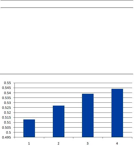

J. RA, K.-J. RHEE
Compared to the backward elimination method, the group
LASSO contains more predictors in the model. In addition, four
separate group LASSO procedures contain different types of
predictors. Besides students’ majo r, total seventeen predictors
are included across four separate models; fourteen variables
(gender, age, area, FEL, MEL, EFI, EST, ME, LRC, LSA, LPT,
LC, STAI, and FLRAS) are selected in the first wave, then ten
variables (place, MEL, ME, LRC, LSA, LP T, and STAI) in the
second wave, nine variab les (gender, income, MEL, ME, LRC,
LS A, E PT, LC , an d S TAI) i n the th ir d wave, and n in e variab les
(age, area, FEL, EST, ME, LRC, LC, STAI, and FLRAS) in the
fourth wave.
Compared to multiple regression and backward elimination
method , the group LASSO i ncludes mor e categorical variables,
such as ar ea, place, and length o f staying abr oad in the fin ali zed
model. However, the results show that four separate group
LASSO methods also contain different sets of predictors in the
model. This might suggest inappropriateness of using the group
LASSO to the repeated measurement.
Results obtained from the LMM show that all the majors and
four continuous explanatory variables (MEL, LST, ME, and
LRC) are included in the finalized model. The results reveal
that TOEIC achievement is positively related with MEL (p
< .05), LST (p < .01), an d LRC (p < .01) but n egatively related
ME (p < .01). Interesting finding is that ME positively affects
TOEIC achievement positi vel y in univariate analysis but affects
TOEIC achievement negatively when considered ME condi-
tional on students’ major, LRC, LST, and MEL.
Once selecting statistically significant predictors in the
model, changes of marginal
2
R
across all possible combina-
tions of predictors are calculated in Table 1. Table 1 shows
that Model 1 only contains MAJOR and LRC in the model.
Model 2 includes MAJOR and LRC with other three predictors
(MS, LST and MEL). To identify which predictors mostly af-
fec t TOEIC achievement, margi nal
2
R
for all possible combi-
nations within Models 2 are also considered.
However, there is less variations among all possible combi-
nations in Model 2. Values of the marginal
2
R
for all possible
combinations of the selected predictors range from .518 to .527.
Model 3 contains five predictors: students’ major, LRC, EST,
ME, and MEL predictors selected from the LMM. Finally,
Model 4 includes all twenty predictors in the model.
Valued of four different marginal
2
R
s for Model 1, Model 2,
Model 3 and Model 4 are .513, .527, .539, and .544, respec-
tively. Figure 2 also describes the changes of marginal
2
R
across four different models.
As shown in Figure 2, there is less chan ges of marginal
2
R
(.005) between Model 4 including nineteen predictors and
Model 3 including 5 predictors. However, compared to changes
of marginal
2
R
from Model 4 to Model 3, changes of mar-
ginal
2
R
from Model 3 to Model 2 is relatively large, .012.
This result suggests that four continuous variables (LRC, ME,
EST, and MEL) should be included in the model.
Conclusion and Discussion
This stu dy examines the relation of TOEIC achievemen t and
twe nt y predictors under four different statistical methods. Dif-
ferent sets of predictors are selected in four different statistical
methods. The results show that there is a strong evidence to
support the existence of relation between TOEIC achievement
and some predictors included in this study. Without considering
Tabl e 1.
Marginal
2
R
for all pos sible combinat ion.
Model Va r iabl es Marginal
2
1 Major, LRC 0.513
2 Major, LRC, ME 0.518
Major, LRC, EST 0.521
Major, LRC, MEL 0.519
Major, LRC, ME, EST 0.527
Major, LRC, ME, MEL 0.527
Major, LRC, EST, MEL 0.527
3 Major, LRC, EST, ME, MEL 0.539
4 All variables 0.544
Figure 2.
Changes of marginal
2
R
.
other predictors, there are much variation in TOEIC reading
achievement among nine different majors. As expected, stu-
dents in medical program have high TOEIC scores compared to
others in different programs. Thus, it is necessar y to in vestigate
predictors which affect growth of TOEIC scores while consid-
ering group difference. Results from this study also show that
LRC (levels of English ability) is a useful variable to explain
and predict TOEIC achievement. Interestingly, LRC is signifi-
cant across four different statistical methods. It makes sense
since the levels of English ability affect TOEIC reading
achievement positively across four waves. However, when
negative rel ation ship between EM an d TOEIC ach ievement h as
emerged when considered ME predictor conditional on other
predictors (major, LRC, EST, and MEL) in the model.
The LMM reveals that there is little variation in the values of
marginal across all possible combinations of predictors in-
cluded in the final model. Among four different statistical
methods, the LMM model seems to be most effective and use-
ful to build a parsimonious model with important and mean-
ingful predictors because it takes into account the repeated
measure ments, which is flexible, and powerful to analyze bal-
anced and unbalanced grouped data. However, these results
must be regarded as very tentative and inconclusive because
this is a search for plausible predictors, not a convincing test of
any theory. Further development based on these results would
require replication with other data and explanation of wh y these
variables appear as predictors of continuity of achievement.
Moreover, this study has some limitations. Besides simply
finding important variables, it is necessary to deal with other
considerations such as optimal size of variables, interaction
effects, and ratio of variables and observations (O’Hara & Sil-
lanpaa, 2009). Another limitation is that the best-fit model
10

J. RA, K.-J. RHEE
among four statistical models is not pursued since the objective
of this r es earch is to test hypotheses based on theories.
Concerning the LASSO method, the group LASSO method
enjoys great computational advantages and excellent perform-
ance, and a number of nonzero coefficient in the LASSO and
the group LASSO method are an unbiased estimate of the de-
gree of freedo m (Efron et al. , 2004) . However, it is necessar y to
consider the LASSO method in the hierarchical structure for
further studies since experiment and survey designs should be
included in the model. Then, the LASSO method in the LM
model framework is useful to explain random effects. Despite
the limitations listed above, this study would contribute to the
field of education as a better way of explaining of relationship
between personal predictors and English ach ievement.
REFERENCES
Agresti, A. (2002). Categorical data analysis (2nd ed.). Boboken, NJ:
John Wiley & Sons.
Agresti, A., & Finlay, B. (1986). Statistical method for the social sci-
ences (2nd, ed.). San Francisco , CA: Dellen.
Akaike, H. (1973). Information theory and an extension of the maxi-
mum likelihood principle. In B. N. Petrov, & F. Csaki (Eds.), Second
international symposium on information theory (pp. 267-281). Bu-
dapest: AcademiaiKiado.
Altman, D. G., & Andersen , P. K. (1989). Boot st r ap investi gation of the
stability of a Coxregression model. Statistics in Medici ne, 8, 771-783.
Bernstein, I. H. (1989). Applied multivariate analysis. New York:
Springer-Verlag.
Bond ell, H. D. , & Rei ch, B. J. (200 8). Simultaneous regression shrink-
age, variable selectionand clustering of predictors with OSCAR. Bio-
metrics, 64, 115-123.
Cohen, J., Cohen, P., West, S. G., & Aiken, L. S. (2003). Appli ed mul-
tipleregression/correlation analysis for the behavioral sciences (3rd
ed.). Ma hwah, NJ: Lawrence Erlbaum.
Derksen, S., & Keselman, H. J. (1992). Backward, forward and step-
wise automated subset selection algorithms. British Journal of Ma-
thema tical and St a tistical Ps y c ho lo gy, 45, 265-282.
Efron, B., Hastie, T., Johnstone, I., & Tib shi rani , R. (2004 ). Lea st an gle
regr ession. The Annals of Statistics, 32, 407-489.
Fan, J., & Li, R. (2001). Variable selection vianonconcave penalized
likelihood and its oracle properties. Journal of the American Statis-
tical Association, 96, 1348-1360.
Foster, D. P., & George, E. I. (1994). The risk inflation criterion for
multiple reg ression. The Anna ls of Sta tis t ic s, 22, 1947-1975.
George, E. I., & McCulloch, R. E. (1993). Variable selection via Gibbs
sampling. Journal of the American Statistical Association, 88, 881-
889.
Gilks, W. R., Wang, C. C, Yvonnet, B., & Coursaget, P. (1993). Ran-
dom effects models for longitudinal data using Gibbs sampling. Bio -
metrics, 49, 441-453.
Hosmer, D. W., & Lemeshow, S. (2000). Applied logistic regression.
New York: Joh n Wiley& Sons.
Laird, N., & Ware, J. H. (1982). Random effec t m od els for lon gi tu din al
data. Biometrics, 38, 963-974.
Mallows, C. L. (1973). Some comments on Cp. Technometrics, 15,
611-675.
Meier, L., van de Geer, S., & Buhlmann, P. (2008). The group lasso for
logistic regression. Journal of Roya l S ta tistica l So ci e ty , B, 70, 53-71.
Menard, S. (1995). Ap p lied logist ic regression analysis (Sage university
paper series on quantitative application in the social sciences, series
no. 10 6) (2nd ed.). ThousandOaks, CA: Sage.
O’Hara, R. B., & Sillanpaää, M. J. (2009). A review of Bayesian vari-
able selection methods: what, how and which. Bayesian Analysis, 4,
85-118.
Orelien.,& Edwards, L. J. (2008). Fixed effect variable selection in
linear mixed models using statistics. Computational Statistics &
Data Analysis, 52 , 1896-1907.
R Development Core Team. (2013). R: A language environment for
statistical computing. Vienna, Austria: The R foundation for statisti-
cal computing. h ttp:// www.R -project.org/
Schwarz, G. (1978). Estimating the dimension of a model. Th e Annals
of Statistics, 6, 461-464.
Tibshi rani, R. (199 6). Regression shrinkage and selection vi a the lasso.
Journal of Royal Statistical So ciety, B, 58, 267-288.
Vonesh, E. F., & Chinchilli, V. M. (1997). Linear and Nonlinear mod-
els for the analysis of repeated measurement. New York: Marcel
Dekker.
Vonesh, E. F., Chinchilli, V. M., & Pu, K. W. (1996).Goodness-of-fit in
generaliz ed nonlinear mixed-effects model. Biometrics, 5 2, 572-587.
Yuan, M., & Lin, Y. (2006).The composite absolute penalties family
for group ed and hierarchical variable selection. Journal of the Royal
Sta tistical Society, B, 68 , 49-67.
Zhang, H. H. Wahba, G., Lin, Y., Voelker, M., Ferris, M., Klein, R., &
Klein, B. (2004). Variable selection and model building via like li-
hood b a sis pu rsui t. Journal of the Amer ica n Sta tisti cal A ssocia tion,
99, 659-672.
Zheng, B. Y. (2000). Summarizing the goodness of fit of generalized
lin ear models for longitudinal data. Statistics in Medicine, 19, 1265-
1275.
Appendix
Group LASSO (R code)
toeic.tr < -as.data.frame(toeic.group[ind[1:225],])
#GROUP LASSO
Cols < -ncol(toeic.tr)-1
index.lasso < -c(rep(0,cols))
numgr < -length(gr)
stg < −1
ltg < -gr[1]
for (i in 1:numgr) {
index.lasso[(stg:ltg)] < -1
if ( I < numgr) {
stg < -stg + gr[i]
ltg < -ltg + gr[I + 1]
}
}
Lamda < -c(2000, 1500, 1000, 500, 1 00 , 10, 1, 0.1, 0.01)
fol d < −10
lamda.lasso < -cvlasso Reg (y~. , to eic.tr, fold, cvind, index.
lasso, l am)
ini.lasso < -grplasso (x = as.matrix(toeic.tr [,-30]),
y = as.matrix(toeic.tr[,30]), index = index.lasso, lamda = lam.
lasso, model = LinReg(), p enscale = sqrt)
lasso.pred < -as.matrix (as.mat rix (toeic.te [,−30]))% * % ini.
Lasso $ coefficients
beta.l as s o < -ini.lasso$coef/sx
OPEN ACCE SS 11