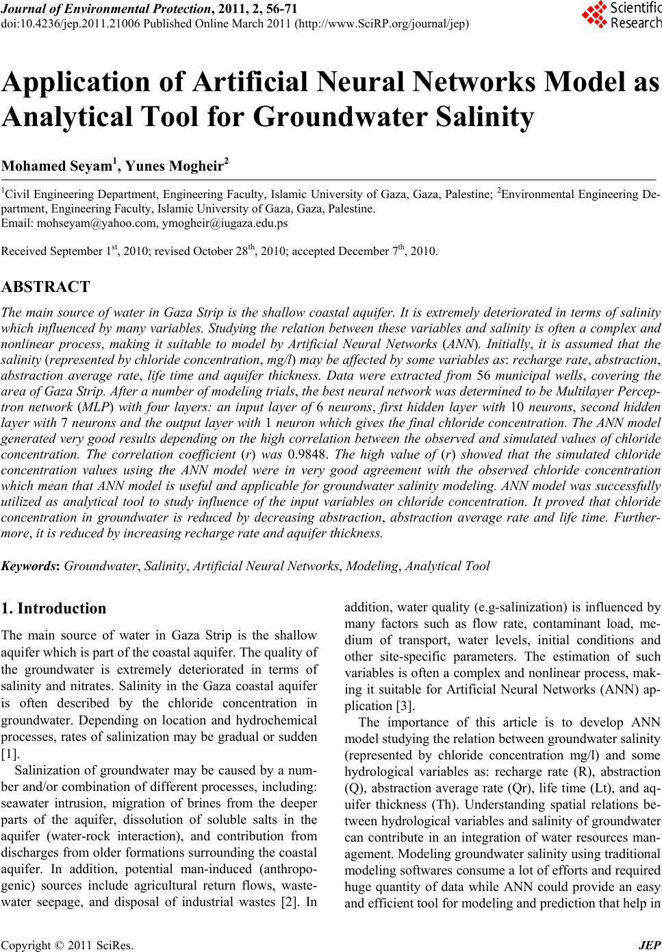
 Journal of Environmental Protection, 2011, 2, 56-71 doi:10.4236/jep.2011.21006 Published Online March 2011 (http://www.SciRP.org/journal/jep) Copyright © 2011 SciRes. JEP Application of Artificial Neural Networks Model as Analytical Tool for Groundwater Salinity Mohamed Seyam1, Yunes Mogheir2 1Civil Engineering Department, Engineering Faculty, Islamic University of Gaza, Gaza, Palestine; 2Environmental Engineering De- partment, Engineering Faculty, Islamic University of Gaza, Gaza, Palestine. Email: mohseyam@yahoo.com, ymogheir@iugaza.edu.ps Received September 1st, 2010; revised October 28th, 2010; accepted December 7th, 2010. ABSTRACT The main source of water in Gaza Strip is the shallow coastal aquifer. It is extremely deteriorated in terms of salinity which influenced by many variables. Studying the relation between these variables and salinity is often a complex and nonlinear process, making it suitable to model by Artificial Neural Networks (ANN). Initially, it is assumed that the salinity (represented by chloride concentration, mg/l) may be affected by some variables as: recharge rate, abstraction, abstraction average rate, life time and aquifer thickness. Data were extracted from 56 municipal wells, covering the area of Gaza Strip. After a number of modeling trials, the best neural network was determin ed to b e Multila yer Percep- tron network (MLP) with four layers: an input layer of 6 neurons, first hidden layer with 10 neurons, second hidden layer with 7 neurons and the output layer with 1 neuron which gives the final chloride concentration. The ANN model generated very good results depending on the high correlation between the observed and simulated values of chloride concentration. The correlation coefficient (r) was 0.9848. The high value of (r) showed that the simulated chloride concentration values using the ANN model were in very good agreement with the observed chloride concentration which mean that ANN model is useful and applicable for groundwater salinity modeling. ANN model was successfully utilized as analytical tool to study influence of the input variables on chloride concentration. It proved that chloride concentration in groundwater is reduced by decreasing abstraction, abstraction average rate and life time. Further- more, it is reduced by increasing recharge rate and aquifer thickness. Keywords: Groundwater, Salinity, Artificial Neural Networks, Modeling, Anal yti c al Too l 1. Introduction The main source of water in Gaza Strip is the shallow aquifer which is part of the coastal aquifer. The quality of the groundwater is extremely deteriorated in terms of salinity and nitrates. Salinity in the Gaza coastal aquifer is often described by the chloride concentration in groundwater. Depending on location and hydrochemical processes, rates of salinization may be gradual or sudden [1]. Salinization of groundwater may be caused by a num- ber and/or combination of different processes, including: seawater intrusion, migration of brines from the deeper parts of the aquifer, dissolution of soluble salts in the aquifer (water-rock interaction), and contribution from discharges from older formations surrounding the coastal aquifer. In addition, potential man-induced (anthropo- genic) sources include agricultural return flows, waste- water seepage, and disposal of industrial wastes [2]. In addition, water quality (e.g-salinization) is influenced by many factors such as flow rate, contaminant load, me- dium of transport, water levels, initial conditions and other site-specific parameters. The estimation of such variables is often a complex and nonlinear process, mak- ing it suitable for Artificial Neural Networks (ANN) ap- plication [3]. The importance of this article is to develop ANN model studying th e relation between groundwater salinity (represented by chloride concentration mg/l) and some hydrological variables as: recharge rate (R), abstraction (Q), abstraction average rate (Qr), life time (Lt), and aq- uifer thickness (Th). Understanding spatial relations be- tween hydrological variables and salinity of groundwater can contribute in an integration of water resources man- agement. Modeling groundwater salin ity usin g tradition al modeling softwares consume a lot of efforts and required huge quantity of data while ANN could provide an easy and efficient tool for modeling and prediction that help in 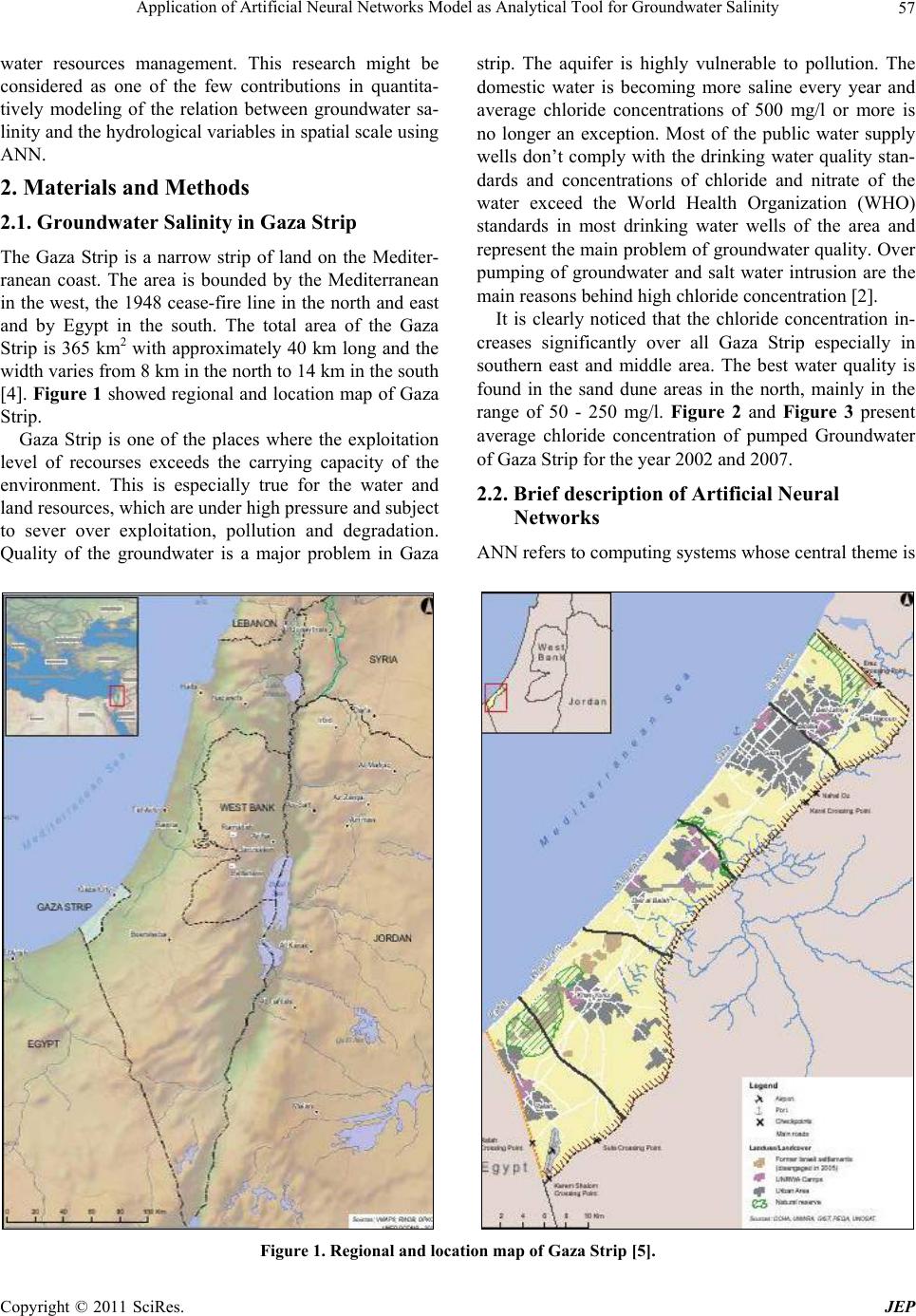 Application of Artificial Neural Networks Model as Analytical Tool for Groundwater Salinity57 water resources management. This research might be considered as one of the few contributions in quantita- tively modeling of the relation between groundwater sa- linity and the hyd rological v ariables in spatial scale using ANN. 2. Materials and Methods 2.1. Groundwater Salinity in Gaza Strip The Gaza Strip is a narrow strip of land on the Mediter- ranean coast. The area is bounded by the Mediterranean in the west, the 1948 cease-fire line in the north and east and by Egypt in the south. The total area of the Gaza Strip is 365 km2 with approximately 40 km long and the width varies from 8 km in the north to 14 km in the south [4]. Figure 1 showed regional and location map of Gaza Strip. Gaza Strip is one of the places where the exploitation level of recourses exceeds the carrying capacity of the environment. This is especially true for the water and land resources, which are under high pressure and subject to sever over exploitation, pollution and degradation. Quality of the groundwater is a major problem in Gaza strip. The aquifer is highly vulnerable to pollution. The domestic water is becoming more saline every year and average chloride concentrations of 500 mg/l or more is no longer an exception. Most of the public water supply wells don’t comply with the drinking water quality stan- dards and concentrations of chloride and nitrate of the water exceed the World Health Organization (WHO) standards in most drinking water wells of the area and represent the main problem of groundwater quality. Over pumping of groundwater and salt water intrusion are the main reasons behind high chloride concentration [2]. It is clearly noticed that the chloride concentration in- creases significantly over all Gaza Strip especially in southern east and middle area. The best water quality is found in the sand dune areas in the north, mainly in the range of 50 - 250 mg/l. Figure 2 and Figure 3 present average chloride concentration of pumped Groundwater of Gaza Strip for the year 2002 and 2007. 2.2. Brief description of Artificial Neural Networks ANN refers to computing systems whose central theme is Figure 1. Regional and location map of Gaza Strip [5]. Copyright © 2011 SciRes. JEP 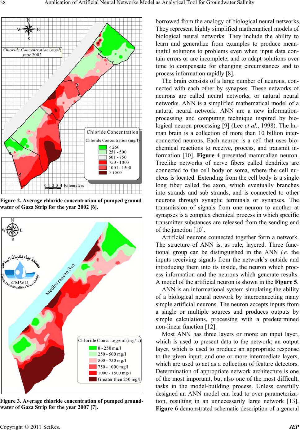 Application of Artificial Neural Networks Model as Analytical Tool for Groundwater Salinity 58 Figure 2. Average chloride concentration of pumped ground- water of Gaza Strip for the year 2002 [6]. Figure 3. Average chloride concentration of pumped ground- water of Gaza Strip for the year 2007 [7]. borrowed from the analogy of biological neural networks. They represent highly si mplified mathematical models of biological neural networks. They include the ability to learn and generalize from examples to produce mean- ingful solutions to problems even when input data con- tain errors or are incomplete, and to adapt solutions over time to compensate for changing circumstances and to process information rapidly [8]. The brain consists of a large number of neurons, con- nected with each other by synapses. These networks of neurons are called neural networks, or natural neural networks. ANN is a simplified mathematical model of a natural neural network. ANN are a new information- processing and computing technique inspired by bio- logical neuron processing [9] (Lee et al., 1998). The hu- man brain is a collection of more than 10 billion inter- connected neurons. Each neuron is a cell that uses bio- chemical reactions to receive, process, and transmit in- formation [10]. Figure 4 presented mammalian neuron. Treelike networks of nerve fibers called dendrites are connected to the cell body or soma, where the cell nu- cleus is located. Extending from the cell body is a single long fiber called the axon, which eventually branches into strands and sub strands, and is connected to other neurons through synaptic terminals or synapses. The transmission of signals from one neuron to another at synapses is a complex chemical process in which specific transmitter substances are released from the sending end of the junction [10]. Artificial neurons connected together form a network. The structure of ANN is, as rule, layered. Three func- tional group can be distinguished in the ANN i.e. the inputs receiving signals from the network’s outside and introducing them into its inside, the neuron which proc- ess information and the neurons which generate results. A model of the artificial neuron is shown in the Figure 5. ANN is an informational system simulatin g the ability of a biological neural network by interconnecting many simple artificial neurons. The neuron accepts inputs from a single or multiple sources and produces outputs by simple calculations, processing with a predetermined non-line ar function [ 1 2]. Most ANN has three layers or more: an input layer, which is used to present data to the network; an output layer, which is used to produce an appropriate response to the given input; and one or more intermediate layers, which are used to act as a collection of feature detectors. Determination of appropriate network architecture is one of the most important, but also one of the most difficult, tasks in the model-building process. Unless carefully designed an ANN model can lead to over parameteriza- tion, resulting in an unnecessarily large network [13]. Figure 6 demonstrated schematic description of a general Copyright © 2011 SciRes. JEP 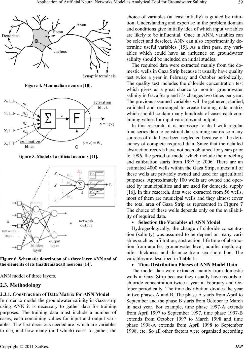 Application of Artificial Neural Networks Model as Analytical Tool for Groundwater Salinity59 Figure 4. Mammalian neuron [10]. Figure 5. Model of artificial neurons [11]. Figure 6. Schematic description of a three layer ANN and of the elements of its (mathematical) neurons [14]. ANN model of three layers. 2.3. Methodology 2.3.1. Construction of Data Matri x for A NN Model In order to model the groundwater salinity in Gaza strip using ANN it is necessary to gather data for training purposes. The training data must include a number of cases, each containing values for input and output vari- ables. The first decisions needed are: which are variables to use, and how many (and which) cases to gather, the choice of variables (at least initially) is guided by intui- tion. Understanding and expertise in the problem domain and conditions give initially idea of which input variables are likely to be influential. Once in ANN, variables can be select and deselect, ANN can also experimentally de- termine useful variables [15]. As a first pass, any vari- ables which could have an influence on groundwater salinity should be included on initial studies. The required data were extracted mainly from the do- mestic wells in Gaza Strip because it usually have quality test twice a year in February and October periodically. The quality test includes the chloride concentration test which gives us a great chance to monitor groundwater salinity in Gaza Strip and it’s changes two times per year. The previous assumed variab les will be gathered, studied, validated and rearranged to create training data matrix which should contain many hundreds of cases each con- taining values for input variables and output. In this research, it is necessary to deal with regular time series data to construct data train ing matrix so many sources of data have been neglected because of the defi- ciency of complete required data. Since that the detailed abstraction records have not been obtained for years prior to 1996, the period of model which include the modelin g and calibration starts from 1997 to 2006. There are an estimated 4000 wells within the Gaza Strip, almost all of these wells are privately owned and used for agricultural purposes. Approximately 100 wells are owned and oper- ated by municipalities and are used for domestic supply [16]. In this research, data were extracted from 56 wells, most of them are municipal wells and they almost cover the total area of Gaza Strip as represented in Figure 7 The choice of these wells depends only on the availabil- ity of required data. Selection the Variables of ANN Model Hydrogeologically, the change of chloride concentra- tion (salinity) was assumed to be depend on many vari- ables such as infiltration, ab straction, life time of ab strac- tion from aquifer, groundwater level, aquifer depth, aq- uifer thickness, and distance from sea shore line. The variables are described in Table 1. Time Distribution Phases of ANN Model Data The model data were extracted mainly from domestic wells in Gaza Strip because they usually have records of chloride concentration twice a year in February and Oc- tober periodically. The time distribution divides the year in two phases A an d B. The phase A starts from April to September and the phase B starts from October to March in next year. For example, time phase 1997-A extends from April 1997 to September 1997, time phase 1997-B extends from October 1997 to March 1998 and time phase 1998-A extends from April 1998 to September 1998, etc. So all other factors were organized according Copyright © 2011 SciRes. JEP 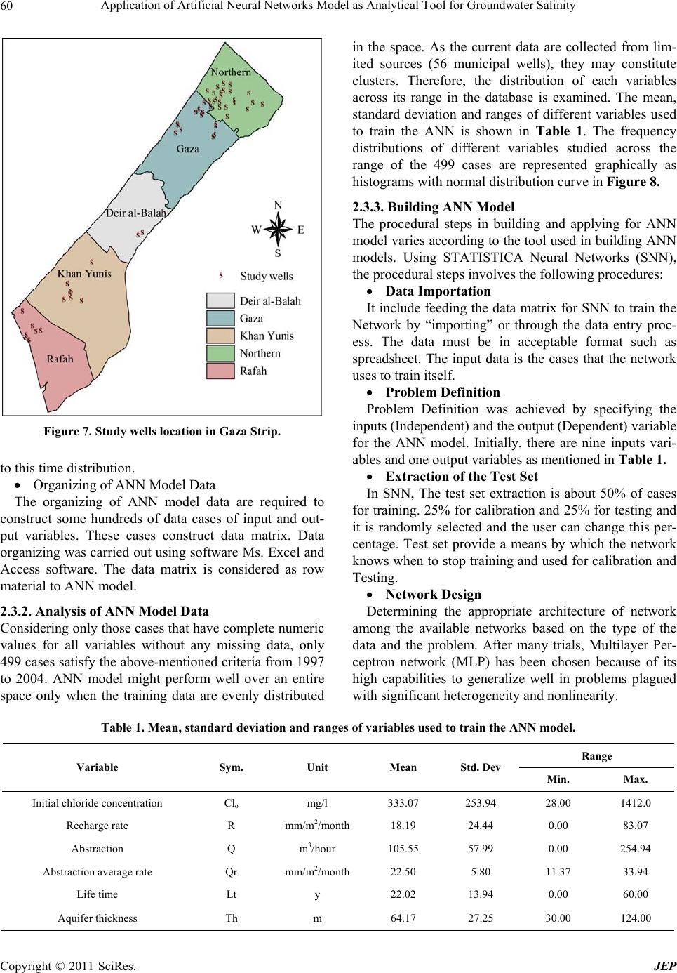 Application of Artificial Neural Networks Model as Analytical Tool for Groundwater Salinity Copyright © 2011 SciRes. JEP 60 in the space. As the current data are collected from lim- ited sources (56 municipal wells), they may constitute clusters. Therefore, the distribution of each variables across its range in the database is examined. The mean, standard deviation and ranges of different variables used to train the ANN is shown in Table 1. The frequency distributions of different variables studied across the range of the 499 cases are represented graphically as histograms with normal distribution curve in Figure 8. 2.3.3. Bui l di n g AN N M odel The procedural steps in building and applying for ANN model varies accord ing to the tool us ed in building ANN models. Using STATISTICA Neural Networks (SNN), the procedural steps involves the following procedures: Data Importation It include feeding the data matrix for SNN to train the Network by “importing” or through the data entry proc- ess. The data must be in acceptable format such as spreadsheet. The input data is the cases that the network uses to train itself. Problem Definition Problem Definition was achieved by specifying the inputs (Independent) and the output (Dependent) variable for the ANN model. Initially, there are nine inputs vari- ables and one output variables as mentioned in Table 1. Figure 7. Study wells location in Gaza Strip. to this time distribution. Extraction of t he Test Set Organizing of ANN Model Data In SNN, The test set extraction is about 50% of cases for training. 25% for calibration and 25% for testing and it is randomly selected and the user can change this per- centage. Test set provide a means by which the network knows when to stop training and used for calibration and Testing. The organizing of ANN model data are required to construct some hundreds of data cases of input and out- put variables. These cases construct data matrix. Data organizing was carried out using software Ms. Excel and Access software. The data matrix is considered as row material to ANN model. Network Design 2.3.2. Analysis of ANN Model Data Determining the appropriate architecture of network among the available networks based on the type of the data and the problem. After many trials, Multilayer Per- ceptron network (MLP) has been chosen because of its high capabilities to generalize well in problems plagued with significant heterogeneity and nonlinearity. Considering only those cases that have complete numeric values for all variables without any missing data, only 499 cases satisfy the above-mentioned criteria from 1997 to 2004. ANN model might perform well over an entire space only when the training data are evenly distributed Table 1. Mean, standard deviation and ranges of variables used to train the ANN model. Range Variable Sym. Unit Mean Std. Dev Min. Max. Initial chloride concentration Clo mg/l 333.07 253.94 28.00 1412.0 Recharge rate R mm/m2/month 18.19 24.44 0.00 83.07 Abstraction Q m3/hour 105.55 57.99 0.00 254.94 Abstraction average rate Qr mm/m2/month 22.50 5.80 11.37 33.94 Life time Lt y 22.02 13.94 0.00 60.00 Aquifer thickness Th m 64.17 27.25 30.00 124.00 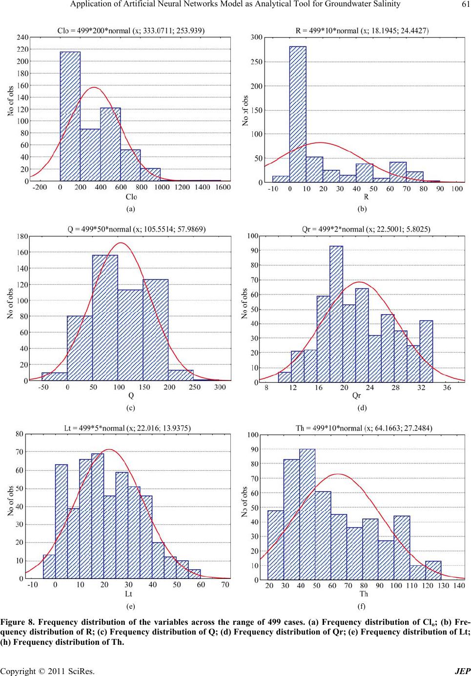 Application of Artificial Neural Networks Model as Analytical Tool for Groundwater Salinity61 (a) (b) (c) (d) (e) (f) Figure 8. Frequency distribution of the variables across the range of 499 cases. (a) Frequency distribution of Clo; (b) Fre- quency distribution of R; (c) Fre quency distribution of Q; (d) Frequency distribution of Qr; (e) Frequency distri bution of Lt; h) Frequency distribution of Th. ( Copyright © 2011 SciRes. JEP 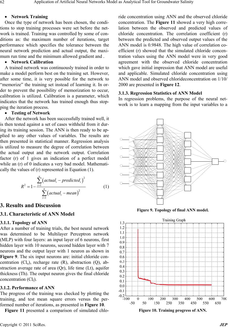 Application of Artificial Neural Networks Model as Analytical Tool for Groundwater Salinity Copyright © 2011 SciRes. JEP 62 Network Training Once the type of network has been chosen, the condi- tions to stop training processes were set before the net- work is trained. Training was controlled by some of con- ditions as: the maximum number of iterations, target performance which specifies the tolerance between the neural network prediction and actual output, the maxi- mum run time and the minimum allowed gradient and . Network Cali bration A trained network was continuously trained in order to make a model perform best on the training set. However, after some time, it is very possible for the network to “memorize” the training set instead of learning it. In or- der to prevent the possibility of memorization to occur, calibration is utilized. Calibration is a parameter, which indicates that the network has trained enough thus stop- ping the iteration pro cess. Testing of Network After the network has been successfully trained well, it is then tested against a set of cases withheld from it dur- ing its training session. The ANN is then ready to be ap- plied to any other values of variables. The results are then presented in statistical manner. Regression analysis is utilized to measure the degree of correlation between the actual output and the network output. Correlation factor (r) of 1 gives an indication of a perfect model while an (r) of 0 indicates a very bad model. Mathemati- cally the values of (r) represented in Equation (1). 2 21 2 1 1 n ii in i i actual predicted R actual mean (1) 3. Results and Discussion 3.1. Characteristic of ANN Model 3.1.1. Topology of ANN After a number of training trials, the best neural network was determined to be Multilayer Perceptron network (MLP) with four layers: an input layer of 6 neurons, first hidden layer with 10 neurons, second hidden layer with 7 neurons and the output layer with 1 neuron as shown in Figure 9. The six input neurons are: in itial chloride con- centration (Clo), recharge rate (R), abstraction (Q), ab- straction average rate of area (Qr), life time (Lt), aquifer thickness (Th). The output neuron gives the final chloride concentration (Clf). 3.1.2. Performance of ANN The progress of the training was checked by plotting the training, and test mean square errors versus the per- formed number of iterations, as presented in Figure 10. Figure 11 presented a comparison of simulated chlo- ride concentration using ANN and the observed chloride concentration. The Figure 11 showed a very high corre- lation between the observed and predicted values of chloride concentration. The correlation coefficient (r) between the predicted and observed output values of the ANN model is 0.9848. The high value of correlation co- efficient (r) showed that the simulated chloride concen- tration values using the ANN model were in very good agreement with the observed chloride concentration which gave initial impression that ANN model are useful and applicable. Simulated chloride concentration using ANN model and observed chlorideconcentration on 1/10/ 2000 are presented in Figure 12 . 3.1.3. Regression Statistics of ANN Model In regression problems, the purpose of the neural net- work is to learn a mapping from the input variables to a Figure 9. Topology of final ANN model. Figure 10. Training progress of ANN. 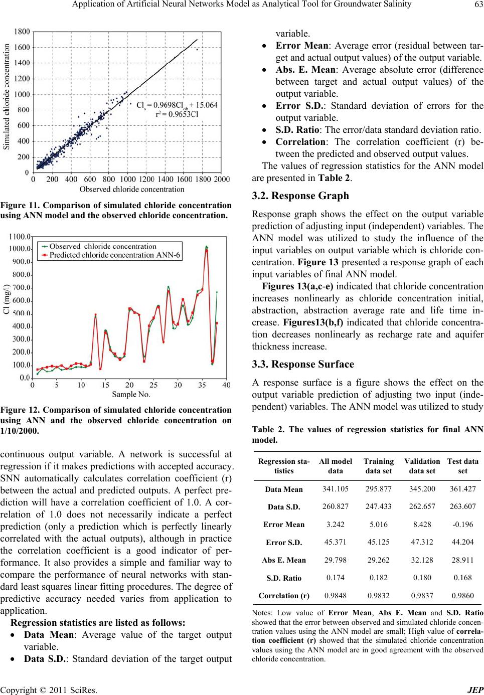 Application of Artificial Neural Networks Model as Analytical Tool for Groundwater Salinity63 Figure 11. Comparison of simulated chloride concentration using ANN model and the observed chloride concentration. Figure 12. Comparison of simulated chloride concentration using ANN and the observed chloride concentration on 1/10/2000. continuous output variable. A network is successful at regression if it makes predictions with accepted accuracy. SNN automatically calculates correlation coefficient (r) between the actual and predicted outputs. A perfect pre- diction will have a correlation coefficient of 1.0. A cor- relation of 1.0 does not necessarily indicate a perfect prediction (only a prediction which is perfectly linearly correlated with the actual outputs), although in practice the correlation coefficient is a good indicator of per- formance. It also provides a simple and familiar way to compare the performance of neural networks with stan- dard least squares linear fitting procedu res. The degree of predictive accuracy needed varies from application to application. Regression statistics are listed as follows: Data Mean: Average value of the target output variable. Data S.D.: Standard deviation of the target output variable. Error Mean: Average error (residual between tar- get and actua l output va lues) of the output variable. Abs. E. Mean: Average absolute error (difference between target and actual output values) of the output variable. Error S.D.: Standard deviation of errors for the output variable. S.D. Ratio: The error/data standard deviation ratio. Correlation: The correlation coefficient (r) be- tween the predicted and observed output values. The values of regression statistics for the ANN model are presented in Table 2. 3.2. Response Graph Response graph shows the effect on the output variable prediction of ad ju sting inp ut (ind ep end ent) variab les. The ANN model was utilized to study the influence of the input variables on output variable which is chloride con- centration. Figure 13 presen ted a response graph of each input variables of final ANN model. Figures 13(a,c-e) indicated that chloride concentration increases nonlinearly as chloride concentration initial, abstraction, abstraction average rate and life time in- crease. Figures13(b,f) indicated that chloride concentra- tion decreases nonlinearly as recharge rate and aquifer thickness increase. 3.3. Response Surface A response surface is a figure shows the effect on the output variable prediction of adjusting two input (inde- pendent) variables. Th e ANN model was utilized to study Table 2. The values of regression statistics for final ANN model. Regression sta- tistics All model data Training data set Validation data set Test data set Data Mean 341.105 295.877 345.200 361.427 Data S.D. 260.827 247.433 262.657 263.607 Error Mean 3.242 5.016 8.428 -0.196 Error S.D. 45.371 45.125 47.312 44.204 Abs E. Mean29.798 29.262 32.128 28.911 S.D. Ratio 0.174 0.182 0.180 0.168 Correlation (r)0.9848 0.9832 0.9837 0.9860 Notes: Low value of Error Mean, Abs E. Mean and S.D. Ratio showed that the error between observed and simulated chloride concen- tration values using the ANN model are small; High value of correla- tion coefficient (r) showed that the simulated chloride concentration values using the ANN model are in good agreement with the observed hloride concentration. c Copyright © 2011 SciRes. JEP 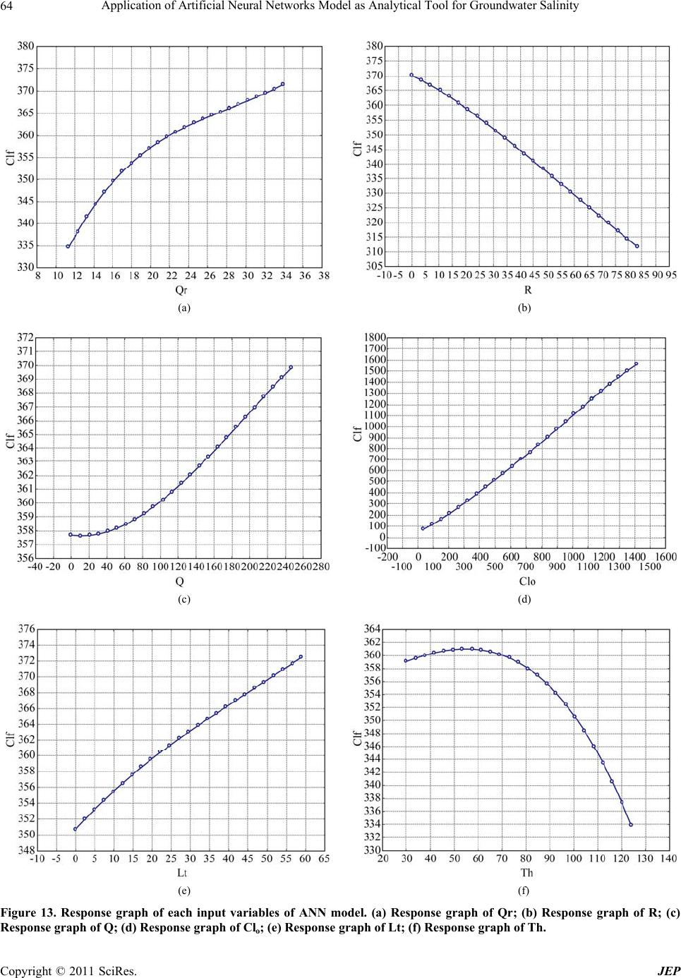 Application of Artificial Neural Networks Model as Analytical Tool for Groundwater Salinity Copyright © 2011 SciRes. JEP 64 (a) (b) (c) (d) (e) (f) Figure 13. Response graph of each input variables of ANN model. (a) Response graph of Qr; (b) Response graph of R; (c) esponse graph of Q; (d) Response graph of Clo; (e) Response graph of Lt; (f) Response graph of Th. R 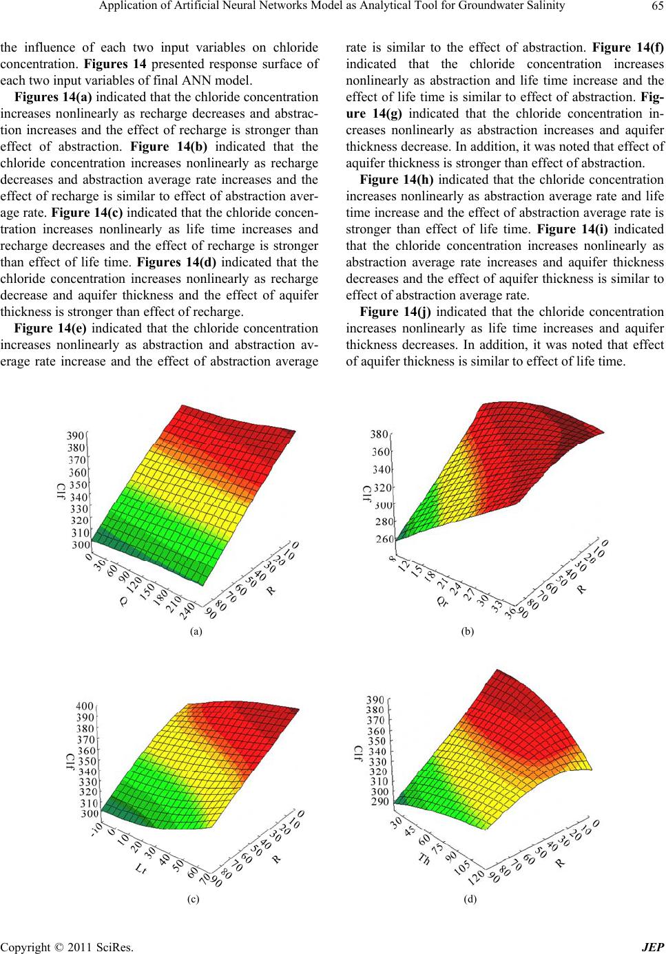 Application of Artificial Neural Networks Model as Analytical Tool for Groundwater Salinity65 the influence of each two input variables on chloride concentration. Figures 14 presented response surface of each two input variables of final ANN model. Figures 14(a) indicated that the chloride concentration increases nonlinearly as recharge decreases and abstrac- tion increases and the effect of recharge is stronger than effect of abstraction. Figure 14(b) indicated that the chloride concentration increases nonlinearly as recharge decreases and abstraction average rate increases and the effect of recharge is similar to effect of abstraction aver- age rate. Figure 14(c) indicated that the chloride concen- tration increases nonlinearly as life time increases and recharge decreases and the effect of recharge is stronger than effect of life time. Figures 14(d) indicated that the chloride concentration increases nonlinearly as recharge decrease and aquifer thickness and the effect of aquifer thickness is stronger than effect of recharge. Figure 14(e) indicated that the chloride concentration increases nonlinearly as abstraction and abstraction av- erage rate increase and the effect of abstraction average rate is similar to the effect of abstraction. Figure 14(f) indicated that the chloride concentration increases nonlinearly as abstraction and life time increase and the effect of life time is similar to effect of abstraction. Fig- ure 14(g) indicated that the chloride concentration in- creases nonlinearly as abstraction increases and aquifer thickness decrease. In add ition, it was noted that effect of aquifer thickness is stronger than effect of abstraction. Figure 14(h) indicated that the chloride concentration increases nonlinearly as abstraction average rate and life time increase and the effect of abstr action average r ate is stronger than effect of life time. Figure 14(i) indicated that the chloride concentration increases nonlinearly as abstraction average rate increases and aquifer thickness decreases and the effect of aquifer thickness is similar to effect of abstraction average rate. Figure 14(j) indicated that the chloride concentration increases nonlinearly as life time increases and aquifer thickness decreases. In addition, it was noted that effect of aquifer thickness is similar to effect of life time. (a) (b) (c) (d) Copyright © 2011 SciRes. JEP 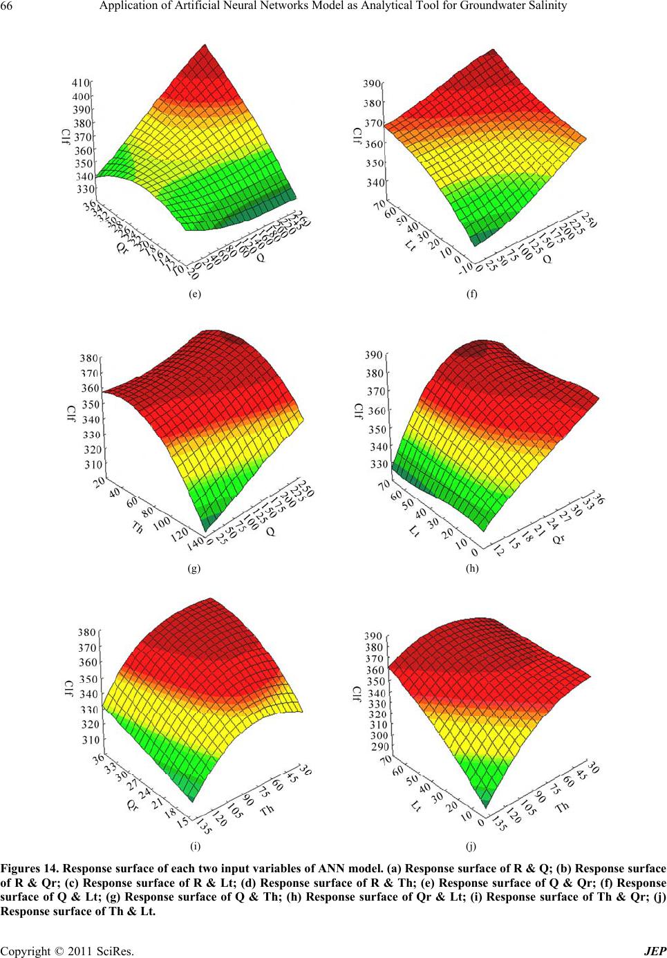 Application of Artificial Neural Networks Model as Analytical Tool for Groundwater Salinity 66 (e) (f) (g) (h) (i) (j) Figures 14. Response surface of each two input variables of ANN model. (a) Response surface of R & Q; (b) Response surface of R & Qr; (c) Response surface of R & Lt; (d) Response surface of R & Th; (e) Response surface of Q & Qr; (f) Response surface of Q & Lt; (g) Response surface of Q & Th; (h) Response surface of Qr & Lt; (i) Response surface of Th & Qr; (j) Response surfac e of Th & Lt. Copyright © 2011 SciRes. JEP 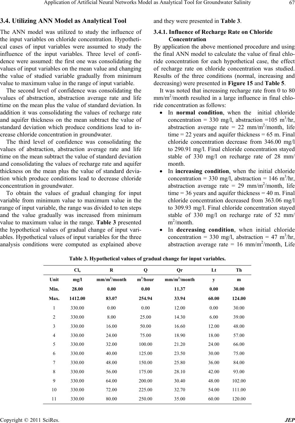 Application of Artificial Neural Networks Model as Analytical Tool for Groundwater Salinity Copyright © 2011 SciRes. JEP 67 3.4. Utilizing ANN Model as Analytical Tool The ANN model was utilized to study the influence of the input variables on chloride concentration. Hypotheti- cal cases of input variables were assumed to study the influence of the input variables. Three level of confi- dence were assumed: the first one was consolidating the values of input variables on the mean value and changing the value of studied variable gradually from minimum value to maximum value in the range of input variable. The second level of confidence was consolidating the values of abstraction, abstraction average rate and life time on the mean plus the value of standard deviation. In addition it was consolidating the values of recharge rate and aquifer thickness on the mean subtract the value of standard deviation which produce conditions lead to in- crease chloride concentration in groundwater. The third level of confidence was consolidating the values of abstraction, abstraction average rate and life time on the mean subtract the value of standard deviation and consolidating the values of recharge rate and aquifer thickness on the mean plus the value of standard devia- tion which produce conditions lead to decrease chloride concentration in groundwater. To obtain the values of gradual changing for input variable from minimum value to maximum value in the range of input variable, the range wa s divided to ten steps and the value gradually was increased from minimum value to maximum value in the range. Tabl e 3 presented the hypothetical values of gradual change of input vari- ables. Hypothetical v alues of inpu t variables fo r the three analysis conditions were computed as explained above and they were presented in Table 3. 3.4.1. I n fluence of Re charge Rat e o n Ch loride Concentration By application the above mentioned procedure and using the final ANN model to calculate the valu e of final chlo- ride concentration for each hypothetical case, the effect of recharge rate on chloride concentration was studied. Results of the three conditions (normal, increasing and decreasing) were presented in Figure 15 and Table 5. It was noted that increasing recharge rate from 0 to 80 mm/m2/month resulted in a large influence in final chlo- ride concentration as follows: In normal condition, when the initial chloride concentration = 330 mg/l, abstraction =105 m3/hr, abstraction average rate = 22 mm/m2/month, life time = 22 years and aquifer thickness = 65 m. Final chloride concentration decrease from 346.00 mg/l to 290.91 mg/l. Final ch loride concentration stayed stable of 330 mg/l on recharge rate of 28 mm/ month. In increasing condition, when the initial chloride concentration = 330 mg/l, abstraction = 146 m3/hr, abstraction average rate = 29 mm/m2/month, life time = 36 years and aquifer thickness = 40 m. Final chloride concentration decreased from 363.06 mg/l to 309.93 mg/l. Final ch loride concentration stayed stable of 330 mg/l on recharge rate of 52 mm/ m2/month. In decreasing condition, when initial chloride concentration = 330 mg/l, abstraction = 47 m3/hr, abstraction average rate = 16 mm/m2/month, Life Table 3. Hypothetical values of gr adual change for input variables. Clo R Q Qr Lt Th Unit mg/l mm/m2/month m3/hour mm/m2/month y m Min. 28.00 0.00 0.00 11.37 0.00 30.00 Max. 1412.00 83.07 254.94 33.94 60.00 124.00 1 330.00 0.00 0.00 12.00 0.00 30.00 2 330.00 8.00 25.00 14.30 6.00 39.00 3 330.00 16.00 50.00 16.60 12.00 48.00 4 330.00 24.00 75.00 18.90 18.00 57.00 5 330.00 32.00 100.00 21.20 24.00 66.00 6 330.00 40.00 125.00 23.50 30.00 75.00 7 330.00 48.00 150.00 25.80 36.00 84.00 8 330.00 56.00 175.00 28.10 42.00 93.00 9 330.00 64.00 200.00 30.40 48.00 102.00 10 330.00 72.00 225.00 32.70 54.00 111.00 11 330.00 80.00 250.00 35.00 60.00 120.00 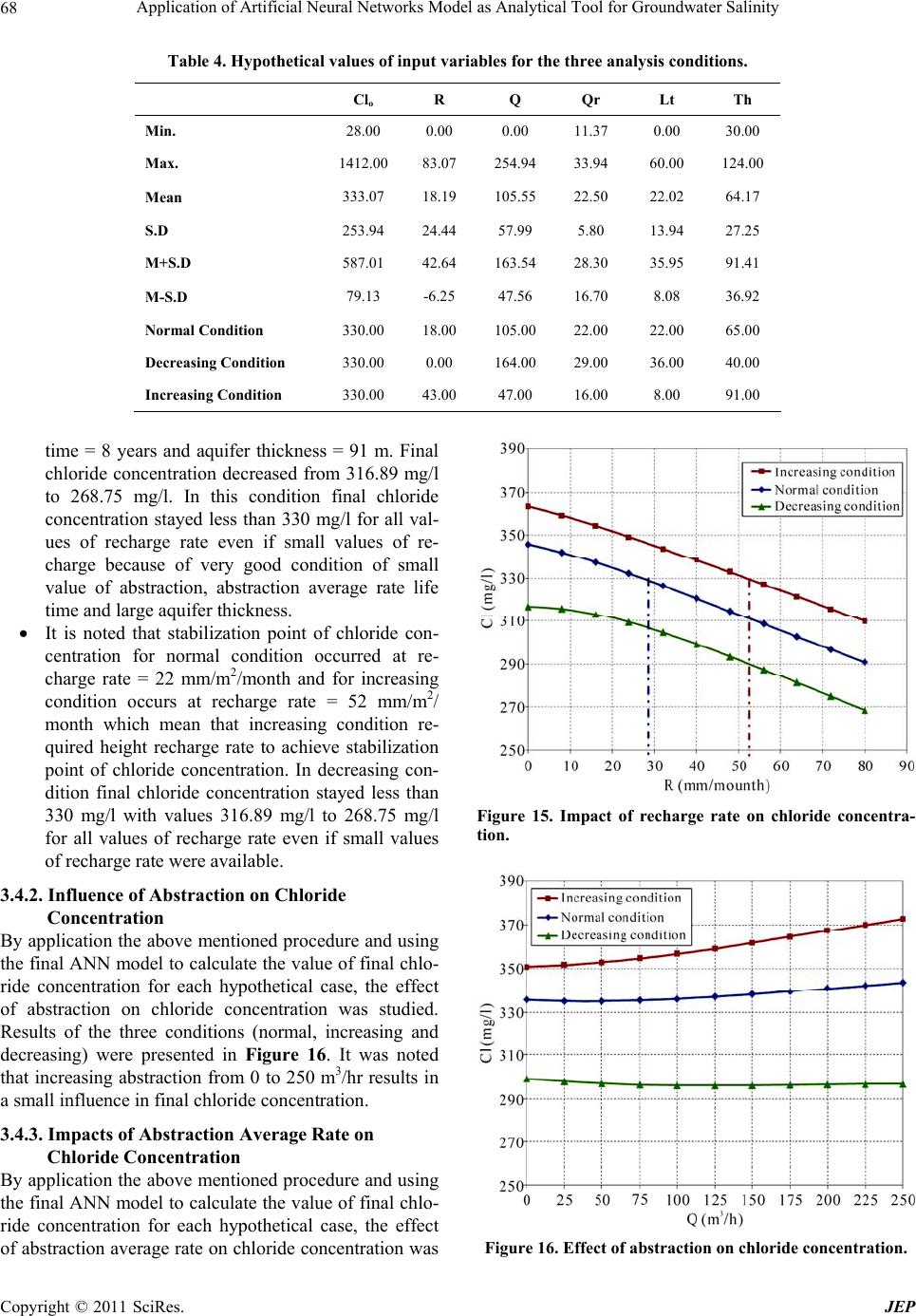 Application of Artificial Neural Networks Model as Analytical Tool for Groundwater Salinity 68 Table 4. Hypothetical values of input var iables for the thr ee analysis conditions. Clo R Q Qr Lt Th Min. 28.00 0.00 0.00 11.37 0.00 30.00 Max. 1412.00 83.07 254.94 33.94 60.00 124.00 Mean 333.07 18.19 105.55 22.50 22.02 64.17 S.D 253.94 24.44 57.99 5.80 13.94 27.25 M+S.D 587.01 42.64 163.54 28.30 35.95 91.41 M-S.D 79.13 -6.25 47.56 16.70 8.08 36.92 Normal Condition 330.00 18.00 105.00 22.00 22.00 65.00 Decreasing Condition 330.00 0.00 164.00 29.00 36.00 40.00 Increasing Condition 330.00 43.00 47.00 16.00 8.00 91.00 time = 8 years and aquifer thickness = 91 m. Final chloride concentration decreased from 316.89 mg/l to 268.75 mg/l. In this condition final chloride concentration stayed less than 330 mg/l for all val- ues of recharge rate even if small values of re- charge because of very good condition of small value of abstraction, abstraction average rate life time and large aquifer thickness. It is noted that stabilization point of chloride con- centration for normal condition occurred at re- charge rate = 22 mm/m2/month and for increasing condition occurs at recharge rate = 52 mm/m2/ month which mean that increasing condition re- quired height recharge rate to achieve stabilization point of chloride concentration. In decreasing con- dition final chloride concentration stayed less than 330 mg/l with values 316.89 mg/l to 268.75 mg/l for all values of recharge rate even if small values of recharge rate were available. 3.4.2. Influence of Abstraction on Chloride Concentration By application the above mentioned procedure and using the final ANN model to calculate the valu e of final chlo- ride concentration for each hypothetical case, the effect of abstraction on chloride concentration was studied. Results of the three conditions (normal, increasing and decreasing) were presented in Figure 16. It was noted that increasing abstraction from 0 to 250 m3/hr results in a small influence in final chloride concen tration. 3.4.3. Impacts of Abstraction Average Rate on Chloride Concentration By application the above mentioned procedure and using the final ANN model to calculate the valu e of final chlo- ride concentration for each hypothetical case, the effect of abstraction average rate on chloride concentration was Figure 15. Impact of recharge rate on chloride concentra- tion. Figure 16. Effect of abstraction on chloride concentration. Copyright © 2011 SciRes. JEP  Application of Artificial Neural Networks Model as Analytical Tool for Groundwater Salinity69 Table 5. Results of ANN model for hypothetical cases stud- ied the effect of recharge rate on chloride concentration. Normal Condition Clo R Q Qr Lt Th Clf 1 330.00 0.00 105.00 22.00 22.00 65.00346.00 2 330.00 8.00 105.00 22.00 22.00 65.00342.11 3 330.00 16.00 105.00 22.00 22.00 65.00337.45 4 330.00 24.00 105.00 22.00 22.00 65.00332.21 5 330.00 32.00 105.00 22.00 22.00 65.00326.58 6 330.00 40.00 105.00 22.00 22.00 65.00320.70 7 330.00 48.00 105.00 22.00 22.00 65.00314.71 8 330.00 56.00 105.00 22.00 22.00 65.00308.67 9 330.00 64.00 105.00 22.00 22.00 65.00302.67 10 330.00 72.00 105.00 22.00 22.00 65.00296.75 11 330.00 80.00 105.00 22.00 22.00 65.00290.91 Increasing Salinity Condition Clo R Q Qr Lt Th Clf 1 330.00 0.00 164.00 29.00 36.00 40.00363.06 2 330.00 8.00 164.00 29.00 36.00 40.00358.88 3 330.00 16.00 164.00 29.00 36.00 40.00354.22 4 330.00 24.00 164.00 29.00 36.00 40.00349.20 5 330.00 32.00 164.00 29.00 36.00 40.00343.91 6 330.00 40.00 164.00 29.00 36.00 40.00338.45 7 330.00 48.00 164.00 29.00 36.00 40.00332.86 8 330.00 56.00 164.00 29.00 36.00 40.00327.19 9 330.00 64.00 164.00 29.00 36.00 40.00321.47 10 330.00 72.00 164.00 29.00 36.00 40.00315.71 11 330.00 80.00 164.00 29.00 36.00 40.00309.93 Decreasing Salinity Condition Clo R Q Qr Lt Th Clf 1 330.00 0.00 47.00 16.00 8.00 91.00316.89 2 330.00 8.00 47.00 16.00 8.00 91.00315.78 3 330.00 16.00 47.00 16.00 8.00 91.00 313.21 4 330.00 24.00 47.00 16.00 8.00 91.00 309.44 5 330.00 32.00 47.00 16.00 8.00 91.00 304.73 6 330.00 40.00 47.00 16.00 8.00 91.00 299.33 7 330.00 48.00 47.00 16.00 8.00 91.00 293.47 8 330.00 56.00 47.00 16.00 8.00 91.00 287.35 9 330.00 64.00 47.00 16.00 8.00 91.00 281.12 10 330.00 72.00 47.00 16.00 8.00 91.00 274.89 11 330.00 80.00 47.00 16.00 8.00 91.00 268.75 studied. Results of the three conditions (normal, increas- ing and decreasing) were presented in Figure 17. It was noted that increasing abstraction average rate from 12 to 35 mm/m2/month results in a large influence in final chloride concentration. 3.4.4. Influence of Life Time on Chloride Concentration By application the above mentioned procedure and using the final ANN model to calculate the valu e of final chlo- ride concentration for each hypothetical case, the effect of life time on chloride concentration was studied. Re- sults of the three conditions (normal, increasing and de- creasing) were presented in Figure 18. It was noted that increasing Life time from 0 to 60 year results in a large influence in final chloride concentration. 3.4.5. Influence of Aquifer Thickness on Chloride Concentration By application the above mentioned procedure and using the final ANN model to calculate the valu e of final chlo- ride concentration for each hypothetical case, the effect of aquifer thickness on chloride concentration was stud- ied. Results of the three conditions (normal, increasing and decreasing) were presented in Figure 19. It was noted that increasing aquifer thickness from 30 to 120 mm/m2/month results in a large influence in final chlo- ride concentration. 4. Conclusions The following conclusions were made based on the re- sults obtained from the current study: 1) A new approach for Groundwater salinity modelling in Gaza Strip utilizing ANN was successfully developed and applied. ANN model was developed to study the relation between groundwater salinity (represented by Figure 17. Effect of abstraction average rate on chloride concentration. Copyright © 2011 SciRes. JEP  Application of Artificial Neural Networks Model as Analytical Tool for Groundwater Salinity 70 Figure 18. Effect of life time on chloride concentration. Figure 19. Effect of aquifer thickness on chloride concen- tration. chloride concentration in groundwater) and some related hydrological factors such as recharge rate (R), abstrac- tion (Q), abstraction average rate (Qr), life time (Lt) and aquifer thickness (Th). 2) The best neural network was Multilayer Perceptron network (MLP) with four layers: an input layer of 6 neu- rons, first hidden layer with 10 neurons, second hidden layer with 7 neurons and the output layer with 1 neuron which gives the final chloride concentration (Clf). 3) The new approach generated very good results de- pending high correlation between the observed and pre- dicted values of chloride concentration. The correlation coefficient (r) between the observed and predicted the output values of the ANN model was 0.9848. The high value of correlation coefficient (r) showed that the simu- lated chloride concentration values using the ANN model were in very good agreement with the observed chloride concentration which mean that ANN model are useful and applicable. 4) The ANN model proved that chloride concentration in groundwater is reduced by decreasing abstraction (Q), abstraction average rate (Qr) and life time (Lt). Further- more, it is reduced by increasing recharge rate (R) and aquifer thickness (Th). 5) Therefore, the current research showed that ANN model can be used in groundwater quality management and it is comparable to other used approaches such as groundwater modelling and statistical modelling. 6) It showed that the strong remedial actions for solv- ing the groundwater deterioration problem in the aquifer of Gaza Strip (salinity) are reducing the abstraction rate and increasing the recharge quantities to the aquifer. REFERENCES [1] Metcalf & Eddy, “Costal Aquifer Management Program,” Final Report: Modeling of Gaza Strip Aquifer, the pro- gram is funded by US Agency for International Devel- opment (USAID) and owned by the Palestinian Water Authority (PWA), Gaza, Palestine, 2000. [2] Coastal Aquifer Management Plan (CAMP), Gaza Coastal Aquifer Management Program, Vol. 1, Task 3, 2000. [3] R. S. Govindaraju, “Artificial Neural Network in Hy- drology,” Journal of Hydrologic Engineering, Vol. 5, No. 2, 2000, pp. 124-137. doi:10.1061/(ASCE)1084-0699(2000)5:2(124) [4] United Nations Environment Programm (UNEP), “Desk Study on the Environment in the Occupied Palestinian Territories,” Switzerland, 2003. [5] United Nations Environment Programm (UNEP), “Envi- ronmental Assessment of the Gaza Strip Following the Escalation of Hostilities in December 2008-January 2009,” Gaza, 2009. [6] Palestinian Water Authority (PWA), (2003). “Groundwa- ter Levels Decline Phenomena in Gaza Strip Final Re- port,” Water Resources and Planning Department-Hy- drology Section, Palestinian National Authority, Gaza, February 2003. [7] Coastal Municipality Water Utility (CMWU), “Annual Report of Wastewater Quality in Gaza Strip for Years 2007 and 2008,” Gaza, Palestine, 2007. [8] S. K. Jain, V. P. Singh and M. T. van Genuchten, “Analysis of Soil Water Retention Data Using Artificial Neural Networks,” Journal Hydrologic Engineering, Vol. 9, No. 5, 2004, pp. 415-420. doi:10.1061/(ASCE)1084-0699(2004)9:5(415) [9] S. Lee, S. Cho and M. Wong, “Rainfall Prediction Using Artificial Neural Networks,” Journal of Geographic In- formation and Decision Analysis, Vol. 2, No. 2, 1998, pp. 233-242. [10] A. Ajith, “Artificial Neural Networks Oklahoma State,” Handbook of Measuring System Design, John Wiley & Sons, Ltd, University, Stillwater, USA, 2005. [11] J. Hola and K. Schabowicz, “Application of Artificial Copyright © 2011 SciRes. JEP  Application of Artificial Neural Networks Model as Analytical Tool for Groundwater Salinity Copyright © 2011 SciRes. JEP 71 Neural Networks to Determine Concrete Compressive Strength Based on Non-Destructive Test,” Journal of civil engineering and management, Vol. 11, No. 1, 2005, pp. 23-32. [12] D. Jeng and H. Cha, “Application of Neural Network in Civil Engineering,” School of Engineering, Griffith Uni- versity Gold Coast Campus, Australia, 2003. [13] K. P. Sudheer, A. K. Gosain, R. D. Mohana and S. M. Saheb, “Modeling Evaporation Using an Artificial Neural Network Algorithm,” Hydrological Processes, Vol. 16, 2002, pp. 3189-3202. doi:10.1002/hyp.1096 [14] M. Claudius and K. Olaf, “Progress Report on Trend Analysis Methods, Tools and Data Preparation (in Par- ticular Artificial Neural Networks (ANN)),” Center for Applied Geoscience, University of Tubingen, Tübingen, 2005. [15] H. Jiang and W. R. Cotton, “Soil Moisture Estimation Using an Artificial Neural Network: A Feasibility Study,” Canadian Journal of Remote Sensing, Vol. 30, No. 5, 2004, pp. 827-839. [16] Palestinian Water Authority (PWA), “National Water Plan,” Final Report, The study is funded by United Na- tion Development Program (UNDP) and owned by the Palestinian Water Authority (PWA), Gaza, Palestine, 2000.
|