Journal of Computer and Communications, 2014, 2, 64-69
Published Online January 2014 (http://www.scirp.org/journal/jcc)
http://dx.doi.org/10.4236/jcc.2014.22012
OPEN ACCESS JCC
Modelling and Analysis on Noisy Financial Time Series
Jinsong Leng
Bradford Street, Mount Lawley, Perth, Australia.
Received November 2013
ABSTRACT
Building the prediction model(s) from the historical time series has attracted many researchers in last few dec-
ades. For example, the traders of hedge funds and experts in agriculture are demanding the precise models to
make the prediction of the possible trends and cycles. Even though many statistical or machine learning (ML)
models have been proposed, however, there are no universal solutions available to resolve such particular prob-
lem. In this paper, the powerful forward-backward non-linear filter and wavelet-based denoising method are
introduced to remove the high level of noise embedded in financial time series. With the filtered time series, the
statistical model known as autoregression is utilized to model the historical times aeries and make the prediction.
The proposed models and approaches have been evaluated using the sample time series, and the experimental
results have proved that the proposed approaches are able to make the precise prediction very efficiently and
effectively.
KEYWORDS
Financial Time Series; Filtering and Denoising; Autoregression; Modelling and Prediction
1. Introduction
In last few decades, the analysis of time series has at-
tracted much attention from statistical and machine
learning perspectives [1,2], with a variety of applications
in different fields [3,4]. For example, the traders of hedge
funds and experts in agriculture are demanding the pre-
cise models to make the prediction of the possible trends
and cycles. Even though a number of techniques and
models are proposed for analyzing financial time series,
however, there are no universal solutions to such specific
application, due to its inherent randomness in nature.
Also it is very difficult to determine which approach or
model is superior to others, since many statistical and
machine learning approaches are application-oriented
methods.
Many real applications, such as the electric signals and
financial time series, consist of high level of white noise
and colored noise, making it almost impossible to build
the appropriate model(s) for prediction and forecasting.
Most of statistical models and machine learning tech-
niques have no capability of noise resistance. Separating
the deterministic time series from the noisy raw signal(s)
is becoming another obstacle to build the effective pre-
diction models.
To address the problems discussed above, several dif-
ferent approaches are proposed in this work. In doing so,
two diversified denoising techniques are introduced and
evaluated through the comparative studies. Also the au-
toregression (AR) model is utilized for modeling and
prediction.
The major task of this work is to develop the statistical
or machine learning (ML) models for analyzing the his-
torical financial time series. Such models should be able
to derive the useful knowledge such as patterns and re-
gularities, trends and cycles, so as to make the precise
prediction. The major contributions of this paper are
summarized as follows:
• Propose two efficient and effective denoising tech-
niques to remove the noise embedded in the time se-
ries i.e., non-line low-pass forward-backward filter
and wavelet orthogonal projection denoising method.
• Build the AR model with the relative low order, and
the excellent performance has been obtained in the
experimental analysis.
• Utilize two new criteria—approximate entropy and
student-t test to assess the performance of filters and
AR model.
The paper is organized as follows: The forward-
backward filter and wavelet denoising method are de-
tailed in Section 2. In Section 3, the AR model is dis-
cussed and the performance criterion is described. In

Modelling and Analysis on Noisy Financial Time Series
OPEN ACCESS JCC
65
Section 4, the experimental results are specified and
evaluated with the sample financial time series available
in book (Analysis of Financial Time Series) [3]. Section
5 concludes the paper.
2. Filters
Normally, the financial time series is embedded with
high level of noise (random trading behaviors), such as
white noise and colored noise. It is very difficult to de-
termine the level of such unknown noise and find the
appropriate filtering techniques that can separate the de-
terministic time series and random events. If the raw
noisy time series is less denoised, the prediction model
performs poorly due to the high level noise; if the noisy
time series is over denoised, the filtered time series loses
some genuine features of raw time series. The conven-
tional time series cannot filter such high level noise such
as financial time series. Indeed, the effective filtering is
dependent on the several factors, e.g., the ability to re-
move the noise, the types of noise, and the thresholds
estimation, etc.
In this paper, two different types of filtering tech-
niques are utilized in this paper: one is the traditional
non-linear low-pass filter with forward and backward
filtering (FBF) processes; another is the wavelet based
denoising method (WLD) for which the time series is
projected into orthogonal basis. Also, the measure crite-
rion known as approximate entropy (ApEn) is considered
to evaluate the performance of proposed filters.
2.1. Forward and Backward Filter
The forward-backward filter (FBF) actually is a matrix
with no-linear processing networks. It utilizes the
second-order matrix SOS and the scale vector G, by
conducting the forward and reverse the filtering pro-
cesses [5]. The scale G defines the weights of input sam-
ples. The SOS and G are defined by:
01 1121011121
02 1222021222
012 012
123456
G[ ]
LL LLLL
bbbaaa
bbbaaa
SOS
bbbaaa
wwwwww



=


=

FBF filters the time series X with the SOS filter de-
scribed by the matrix SOS and the vector G. After filter-
ing in the forward direction, the filtered sequence is then
reversed and run back through the filter. In this project,
the Butterworth second-order filtering is used for filter-
ing the time series.
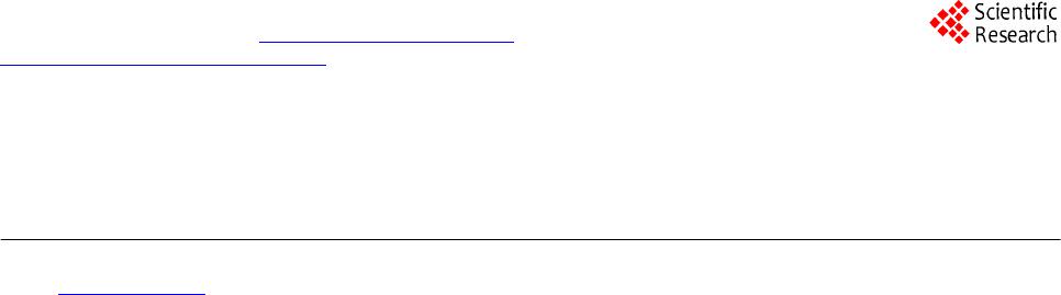
The example of FBF filtering process with the finan-
cial time series is illustrated in Figure 1.
2.2. Wavelet-Based Denosing
Wavelet theory is an emerging new signal processing
technique in recent two decades [6,7], which is called the
mathematical microscope due to it high recognition ac-
curacy in both time domain and frequency spectrum.
With the scaling factor a (dilation factor) and translation
parameter b, a, b ∊ R, and a ≠ 0. The prototype wavelet
is scaled and translated. The wavelet function can be
expressed as:
( )
1
,tb t aba
a
−

Ψ=Ψ


1/ a
is the normalized factor, so as to make sure for
all a, b, Ψ() has the unit energy.
The concept of multiresolution was proposed by Mal-
lat and Meyer in 1989 [8], meaning that one signal can
be decomposed into the orthogonal projections and can
also be fully reconstructed. The components of the de-
composition are divided into the approximation (a) and
details (d) at different levels. The approximation repre-
sents the major feature of the signal and the details de-
scribe the detailed changes and noise. The time series can
be denoised by removing some ingredients from the pro-
jections in details.
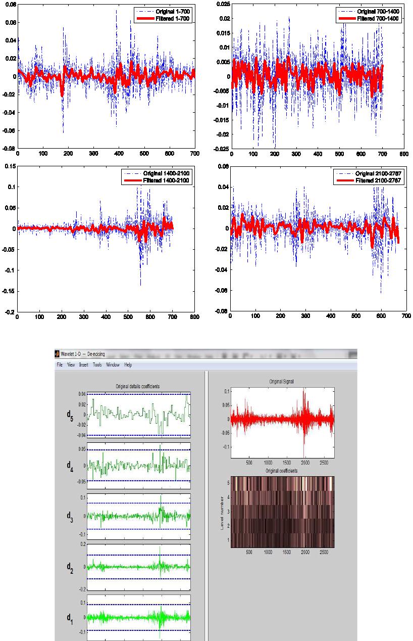
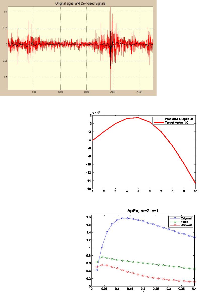
The example of wavelet denoising is given in Figure s
2 and 3.
2.3. Performance Measurement
To evaluate two filters proposed above, two measure-
ments are introduced: 1). One indicator is the fit rate of
autoregression model (AR), the details about AR model
are available in Chapter 3. 2). Another criterion known as
the approximate entropy (ApEn) [9] is also introduced.
The major ability of ApEn is to evaluate the time se-
ries by quantifying the amount of regularity and the un-
predictability of fluctuations. The successful applications
have been found in EEG signal diagnosis [10] and in
financial time series [11]. In [11], it was reported that the
uncertainty events such as the Asian financial crisis can
be detected by analyzing Hang Seng index. There are
two parameter m and r in ApEn. The value of m is be-
tween 2 - 3, and the value of r is about 0.2 × σ (σ is the
value of standard deviation of the time series).
The smaller of ApEn, the better regularity and trends
of the time series.
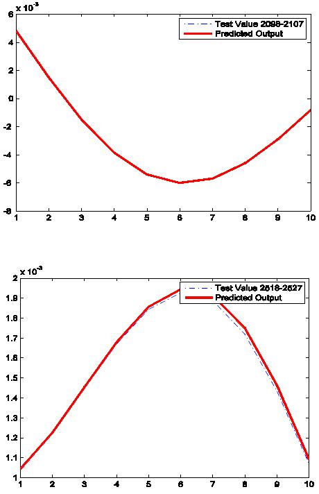
Here, an example is given to assess the performance of
two filters using AR model and ApEn. Firstly, I compare
the quality of filtering with time series L0 using AR(p)
model, detailed as below (FPE—final prediction error,
MSE—mean square error):
• For original signal L0, the results with AR (6) are: Fit
to estimation data—0.3754%, FPE—0.0002323, MSE
—0.0002308. Even AR with order of 30, the results

Modelling and Analysis on Noisy Financial Time Series
OPEN ACCESS JCC
66
Figure 1. Original and filtered times series (FBF).
Fgure 2. Approximate and details of times series.

Modelling and Analysis on Noisy Financial Time Series
OPEN ACCESS JCC
67
Figure 3. Original and filtered times series (Wavelet).
are still very poor: Fit to estimation data—1.202%,
FPE—0.0002344, MSE—0.00022 7.
• For the forward-backward filtered L0, the results with
AR (6) are: Fit to estimation data—99.98%, FPE—
1.557e-12, MSE—1.548e-12.
• For the wavelet-based denoised L0, the results with
AR (6) are: Fit to estimation data—99%, FPE—
6.884e-10, MSE—6.842e-10.
• It is almost impossible to build the AR model with the
original signal (fit rate (r) is too low, 0 < r < 22%).
After filtering using FBF or wavelet, AR(p) model
can be built and used to make the prediction. The
performance (almost 100% fit rate) of AR is excellent
using the filtered time series by FBF or wavelet.
Also two filters can be evaluated by another criterion
ApEn. As shown in Figure 4, we can find the ApEn val-
ue of original signal is significant bigger at r = 0.2. Fig-
ure 5 suggests that wavelet-based denoising is slightly
better than that of forward-backward filter. However, AR
model indicates that FBF outperforms a little better than
wavelet-based denoising method.
Due to space limit, I only use the filtered datasets by
FBF to conduct the model training and prediction.
3. Model
3.1. Autoregression
Let {r0, r1,…, rt, …} be a time series, the pth order au-
toregressive polynomial model AR(p) model [1,2] is de-
fined by:
( )
0 1111tpt ptpt pt
rtrrrra
−−−−
=∅+∅ +…+∅+∅ +…+∅+
where p is a non-negative integer and ∅p are the coeffi-
cients in the autoregressive model,
{ }
t
a
is assumed to
be a white noise series with mean zero and variance
2
t
a
.
The parameters of the AR(p) can be estimated by sev-
Figure 4. Predicted output and target value (1).
Figure 5. ApEn value of original and filtered signal.
eral ways to replace the theoretical covariance, including
the forward-backward approach, the Least Squares me-
thod, the Yule-Walker method, etc. In this project, the

Modelling and Analysis on Noisy Financial Time Series
OPEN ACCESS JCC
68
forward-backward approach is used to estimate the pa-
rameters of the AR(p) model. The AR(p) can be trained
and validated by sample time series. Once the AR(p) is
built, it can be used to predict the future trends and
cycles.
3.2. Student-T Test
One statistical criterion known as Student-t test is used to
quantify the “goodness” of the prediction. This is the
statistical criterion to make a test decision for paired time
series. The test decision for the null hypothesis is to be
made in terms of the acceptance or rejection (h: 0 or 1)
and the confidence level (p-value). For example, if p =
0.95, the probability of rejecting null hypothesis is only
5%, and thus the prediction will be regarded as the high
quality.
4. Experiments
There are two parameters in AR to be tuned, i.e., the
length of prediction (output), and the order p in AR. The
order of p is required to be tuned in advance. Also it is
not easy to evaluate the quality of the AR model, I in-
clude a function to calculate the Student-t test values and
thus can adjust the order of AR model easily. The order
of p is tuned according to the student-t p-values. After
several times trials, I find the best solution to all time
series in datasets when the order of p is 18. Also I found
that AR model can predict 10 - 15 days perfectly, but it is
getting worse when the prediction period is more than 20
days. So I define the prediction period is 10 days.
The last 10 records in the time series in dataset 1 are
retained for testing, while the rest of the records (total
length - testing length) is used for training and valida-
tion.The prediction and the filtered testing is a good
matching, as shown in Figure 4.
The p-value of this experiment is excellent (0.998),
which indicates that the prediction of AR model is pre-
cisely matched to testing records.
To further evaluate the proposed methods, additional
testing is conducted by making prediction at any point of
time series.
For example, the financial time series (1 - 2097) is
used for training and next 10 days (2098-2107) as the
testing data, as shown in Figure 6. The related p-values
are 0.982 and MSE 1.81e - 08.
Another example is given in Figure 7, the related
training data are from 1 to 2157 and the testing data are
from 2158 to 2167. From Figures 6 and 7, we can see
the predicted data and testing data is matched precisely.
The related p-values are 0.915 and MSE 4.03e−09.
5. Conclusions
In this paper, several methods have been used to com-
Figure 6. Predicted output and target value (2).
Figure 7. Predicted output and target value (3).
plete the tasks, i.e., two denoising filters, AR prediction
models, and two assessment criteria. The approaches of
two filters (filtering and wavelet denoising) are proposed
from different perspectives.
The advantage of using different approaches and mod-
els can provide alternative solutions and the comparative
studies to this specified application. The quality measure
known as approximate entropy is introduced to assess the
quality of preprocessing methods; another statistical cri-
terion known as Student-t test is used for quantifying the
prediction models. The software codes for all models and
approaches have been developed and tested with two
sample datasets under Matlab. The experimental results
and related performance are excellent.
In summary, there are some challenges and difficulties
in this work, outlined as follows:
• Further analysis is needed to analyze: which filter is
better?
• The back-propagation neural networks is to be consi-
dered as alternative model, so as to provide alterna-
tive
• The use of different portfolio analysis models is

Modelling and Analysis on Noisy Financial Time Series
OPEN ACCESS JCC
69
needed to conduct the analysis folio optimization.
In a word, it is clear that the satisfactory results have
been obtained; indicating that the proposed approaches
and criteria are very effective in analyzing the big
finance time series. If the prediction models can be
trained using more systematic samples (different cycles
and scenarios), the trained models should be more smart
and adaptive.
REFERENCES
[1] G. U. Yule, “On a Method of Investigating Periodicities
in Disturbed Series,” Philosophical Transactions of the
Royal Society of London, Vol. 226, 1927, pp. 267-298.
http://dx.doi.org/10.1098/rsta.1927.0007
[2] T. C. Fu, “A Review on Time Series Data Mining,” En-
gineering Applications of Artificial Intelligence, Vol. 24,
2011, pp. 164-181.
http://dx.doi.org/10.1016/j.engappai.2010.09.007
[3] R. S. Tsay, “Analysis of Financial Time Series,” John
Wiley & Sons, Inc., New York, 2010.
[4] D. B. Percival and A. T. Walden, “Wavelet Methods for
Time Series Analysis,” Cambridge University Press,
Cambridge, 2000.
http://dx.doi.org/10.1017/CBO9780511841040
[5] F. Gustafsson, “Determining the Initial States in For-
ward-Backward Filtering,” IEEE Transactions on Signal
Processing, Vol. 44, No. 4, 1996, pp. 988-992.
http://dx.doi.org/10.1109/78.492552
[6] I. Daubechies, “Ten Lectures on Wavelets,” Society for
Industrial and Applied Mathematics, Philadelphia, 1992.
http://dx.doi.org/10.1137/1.9781611970104
[7] C. K. Chui, “An Introduction to Wavelets,” Academic
Press, 1992.
[8] S. G. Mallat, “A Theory for Multiresolution Signal De-
composition: The Wavelet Representation,” IEEE Trans-
actions on Pattern Analysis and Machine Intelligence,
Vol. 11, 1989, pp. 674-693.
http://dx.doi.org/10.1109/34.192463
[9] S. M. Pincus, “Approximate Entropy as a Measure of
System Complexity,” National Academy of Sciences of
the United States of America, Vol. 88, No. 6, 1991, pp.
2297-2301. http://dx.doi.org/10.1073/pnas.88.6.2297
[10] S. M. Pincus, I. M. Gladstone and R. A. Ehrenkranz, “A
Regularity Statistic for Medical Data Analysis,” Journal
of Clinical Monitoring and Computing, Vol. 7, No. 4,
1991, pp.335-345.
[11] S. M. Pincus and E. K Kalman, “Irregularity, Volatility,
Risk, and Financial Market Time Series,” Proceedings of
the National Academy of Sciences, Vol. 101, No. 38,
2004, pp. 13709-13714.
http://dx.doi.org/10.1073/pnas.0405168101