Enhancement Technique of Image Contrast using New Histogram Transformation
OPEN ACCESS JCC
mented in consumer electronics, such as digital TV, be-
cause the method tends to produce undesirable artifacts.
Hence, many improved methods have been proposed to
overcome these drawbacks. They are brightness preserv-
ing bi-histogram equalization (BBHE), dualistic sub-
image histogram equalization (DSIHE), minimum mean
brightness error bi-histogram equalization (MMBEBHE),
recursive mean-separate histogram equalization (RMSHE),
recursive sub-image histogram equalization (RSIHE),
mul ti -peak histogram equalization with brightness pre-
serving (MPHEBP), and dynamic histogram equalization
(DHE). On the other hand, another popular contrast en-
hancement scheme is histogram specification. This tech-
nique enables us to match the histogram of input image
close to the histogram of target image. However, speci-
fying the output histogram is not a smooth task as it va-
ries from image to image. Hence, several researches have
been proposed on improvement of histogram specifica-
tion. They are dynamic histogram specification (DHS),
Histogram specification with Gamma distribution (HSGD),
image fusion histogram specification (IFHS), and auto-
matic exact histogram specification (AEHS).
However, there are some problems when we have used
the histogram equalization (HE) to improve the contrast
of the image. First, the HE method does not take the
mean brightness of an image into account. Second, the
HE method may result in over enhancement and satura-
tion artifacts due to the stretching of the gray levels over
the full gray level range. Third, the HE method always
yields the middle gray level regardless of the input image,
and cause undesirable artifacts. Therefore, in order to
improve these problems, we have decided in advance the
target images and then we use the histogram specifica-
tion method to an input image to get an image similar
with target image. But, it is difficult that we determine in
advance the appropriate target image. Hence, it is re-
quired to a new contrast enhancement method robust to
illumination changes.
Hence, in order to solve these problems at the same
time, we try to propose a new image enhancement me-
thod that uses a new histogram transformation. In the
Section 2, in order to enhance the image contrast, we
have considered new adaptive histogram transformation
combining histogram equalization and histogram speci-
fication. In the Section 3, we presented experimental
results that is able to demonstrate the effectiveness of the
proposed method in comparison to a few existing me-
thods quantitatively. And in the Section 4, we mentioned
the conclusion of my paper.
2. Contrast Enhancement
2.1. CDF Transformation
Here we will propose a technique that can improve the
contrast of an image by using a combination of Histo-
gram Equalization (HE) and Histogram Specification
(HS). This technique can be thought as the transforma-
tion that converts the values in the ranges between 0 and
1 given by histogram equalization of input image into
pixel values of particular output image by using the spe-
cified cumulative distribution function (CDF) to achieve
a well illuminated image. In our case, we adaptively se-
lect the CDF so that the contrast of image can automati-
cally achieve an optimal level.
First, we assume to have an input image I(x,y) with N
pixels and a total number of L gray levels, e.g., 256 gray
levels for an 8-bit image. We transform the distribution
of the pixel intensity values in the image I(x,y) into a
uniform distribution on interval [0,1] by using the histo-
gram equalization defined as the following formula. For
a grey level of k, k = 0, 1, ⋯, L-1, a new transformed one
uk is defined by
0
,[0, ,L 1]
ki
ki
n
uk
N
=
= ∈−
∑
. (1)
where ni denotes the number of pixels in I(x,y) with the
grey level value i. Equation (1) defines a mapping of the
pixel’ intensity values from their original range [0,⋯,L-1]
to the domain of [0,1].
Second, if the distribution of desired target image ITA
is specified, we define its probability density function
(PDF) and CDF as follows:
0
G(z)(v)dv,z[0,L 1]
z
z
p= ∈−
∫
. (2)
Third, we try to find a new value knew corresponding
with uk such that
0
uG(k )(v)dv
new
k
k newz
p= =
∫
. (3)
But, since a new value knew is continuous value scaled
on an interval [0, L-1], we should take a Gauss bracket
integer [knew + 0.5].
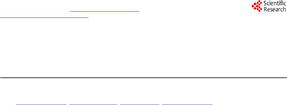
Here, the procedure that we have considered so far
would be expressed as the following example picture.
Figure 1 shows the density histogram of a given image,
its equalized histogram & specified CDF, and the density
histogram of output image.
Furthermore, we consider the three types of density
histogram structures in order to determine adaptively a
proper CDF form in our CDF transformation.
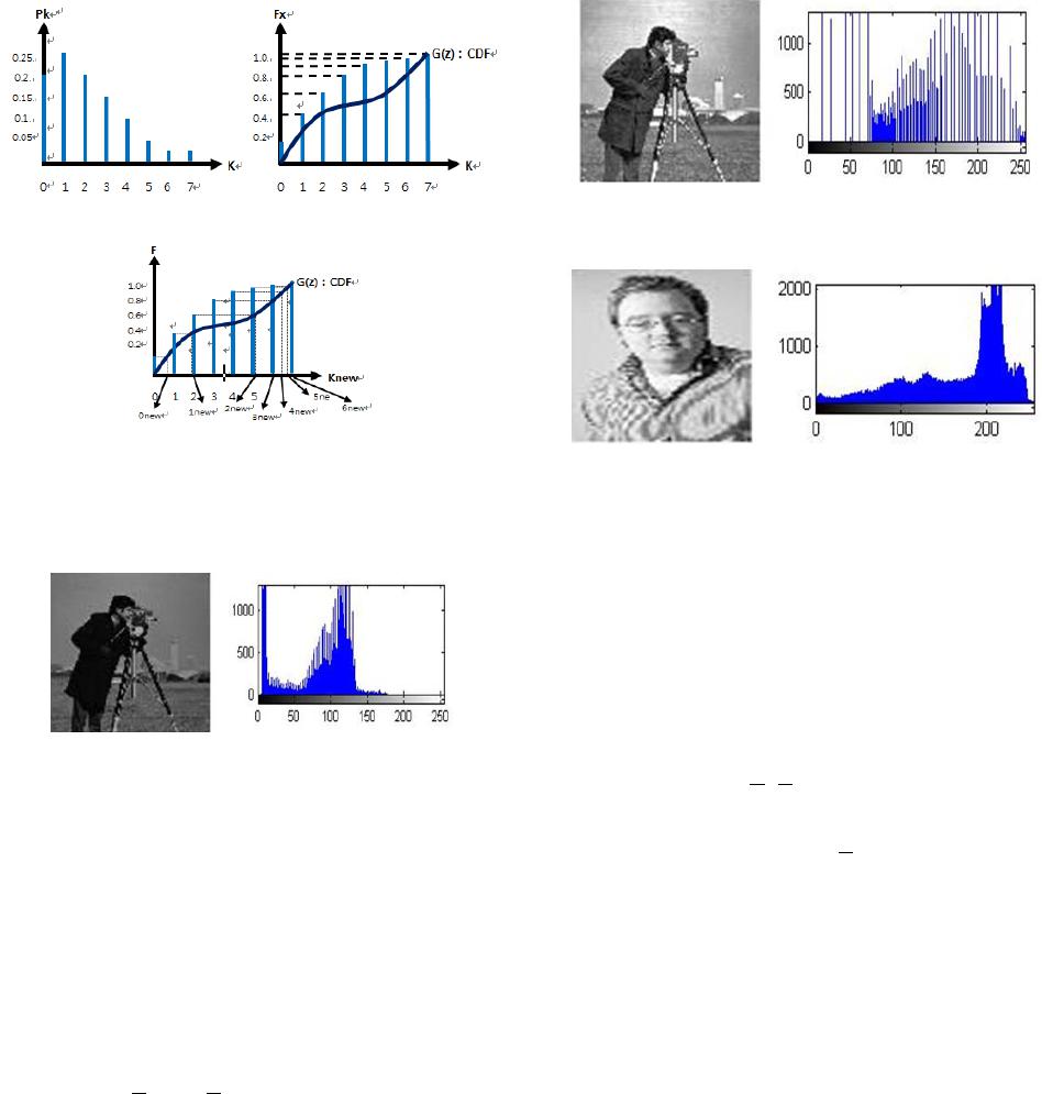
2.2. Skew Histogram to the Right
When it is given a dark image like as the following ex-
ample image in Figure 2, its density histogram has a
form skewed to the right.
In this case, the average of the gray values of a given
image is smaller than the average value (N + 1)/2 of
symmetrical distribution. Furthermore, in order to im-