 Journal of Service Science and Management, 2011, 4, 79-85 doi:10.4236/jssm.2011.41011 Published Online March 2011 (http://www.SciRP.org/journal/jssm) Copyright © 2011 SciRes. JSSM 79 Agency Cost under the Restriction of Free Cash Flow Junhong Chu Department of Finance Zhuhai Campus, Jinan University, Zhuhai, China. Email: jhchu@126.com Received November 12th, 2010; revised December 22nd, 2010, accepted December 24th, 2010. ABSTRACT Agency cost theory is an important branch of capital structural theory. Free cash flow has significant impact on agency cost. The combination of research on these two fields would help to build and extend the theoretical system. Based on agency cost theory, the present study firstly categorized the characteristics of free cash flow as well as the statistical methodologies. Furthermore, the existence of investing free cash flow in agency cost was proved by a model. Then free cash flow was introduced into agency cost theory as restriction, the analysis shows that it will change agency cost, in turn, will have an impact on the relationship between agency cost and capital structure, finally, will influence the opti- mal capital structure point to maintain the equilibrium. Concretely, with the increasing free cash flow, correspondingly, debt proportion will decrease. Keywords: Capital Structure, Free Cash Flow, Agency Cost, Non-Pecuniary Benefit 1. Introduction Agency cost theory, financial contract theory, signaling model and new pecking order theory are the main branches of new capital structure theory. Financial con- tract theory focuses on restricting stockholders’ behavior by contract and solving the conflict between stockholders and creditors. Signaling model and new pecking order theory center on solving the conflict between investors and managers. These two types of conflict are the main conflict in business organizations. Agency cost theory considers how equilibrium is reached in both types of conflict and how capital structure is formed, which is more theory is more comprehensive than the previous two to some degree. In the famous paper “Theory of the Firm: Managerial Behavior, Agency Costs and Ownership Structure” in 1976, Jensen argues that the ownership of outsiders will generates agency costs [1,2]. However, Jensen’s model is too perfect to be actualized. In his model, there is an im- portant precondition: the manager-owner can use up all value of the firm as non-pecuniary benefits [3]. While in fact, the value of firm contains many compositions which can’t be abused, so it might be better to introduce a new variable to modify the original model. Free cash flow could be one. 2. Literature Review Jensen acknowledged the important role of free cash flow himself. He considered that the free cash flow can represent agency costs to a great degree, so in stock market the announcement of free cash flow might lead to explicit price fluctuation. However, he didn’t introduce it into his classical model to provide a reasonable explana- tion. Figure 1 is the original model in Jensen’s paper. The y-axis V represents the value of firm, and the x-axis F represents consumed, and Uj (j = 1, 2, 3) represents owner’s indifference curves between wealth and non- pecuniary benefits. When the manager-owner has 100 percents of the equity, the slope of VF is −1, the value of the firm will be V* where indifference curve U2 is tan- gent to VF, and the level of non-pecuniary benefits con- sumed is F*. Supposing the owner sells a fraction of the firm, 1 − α, and holds α for himself, the slope of constraint line will change to –α. As a result, the deal will bargain on the price of V’, as shown in the Figure 1, where the line with slope –α tangent the indifference curve on the location of the constraint line. Now the value of the firm is F’, which This paper is sponsored by the Incubating Program for Outstanding and Creative Talented Youths in Guangdong Colleges and Universities (No.: WYM08050).  Agency Cost under the Restriction of Free Cash Flow 80 Figure 1. The original model of Jensen. is lower then F*. As Jensen stated, selling to outsiders brings about the drop of value, which is a kind of agency costs. Jensen called it the agency cost associated with outside equity. In this model, a very important condition is that the manager can choose the level of non-pecuniary benefits “free”, which means every point on the VF is accessible. But in reality, can this condition be fulfilled? Similar with outside stock ownership, enterprise debt consequentially leads to internal managers’ acts of agency to funds of outside creditors, which generates agency cost too. Jensen discussed the agency cost of debt in a simple case. Besides agency cost in Jensen’s paper, Myers analyzed agency cost of debt from the other per- spective. Although they used different analysis methods and models, they drew similar conclusion that agency cost of debt exists and increases with the amount of debt [2]. As mentioned above, outside stock ownership and debt will bring agency cost to enterprises. Thus, the amount of outside stock ownership and debt will determine the agency cost paid by the enterprise and in turn determine the value of enterprise when the scale of enterprise re- mains the same. Adopting this argument, Jensen and Meckling pre- sented the theoretical framework that agency cost deter- mines capital structure. Assuming other conditions as constant value, the value of enterprise is Vm when agency cost is 0 which is an ideal state. Since agency cost is the only antecedent of the value of enterprise, then the maximum of enterprise value will be the point of the lowest agency cost E*, on which value of enterprise is Vm − A T(E*). The point represents the optimal capital structure under the condi- tion of enterprise scale and financing scale. This maxi- mum point of enterprise value is achieved by adjusting capital structure, which supports the proposition pre- sented by Jensen and Meckling that capital structure de- termines enterprise value. 3. Propositions Development The value of firm contains several kinds of components, such as real estate, equipment, brand and cash. In these components, only cash can be used by the manager freely. In fact, not all cash could be “freely” used. The part that can be used freely is described as free cash flow. This is the essence of free cash flow. According to this essence, there are several different explicit definitions of free cash flow. Jensen defined that free cash flow is cash flow in ex- cess of that required to fund all projects that have posi- tive net present values when discounted at the relevant cost of capital. His definition is difficult to be executed in accounting, because there is no way to judge whether a project has net present value when the project is just set- tled. Rubin used the similar definition with Jensen. Their definition can be expressed as below [4]: FCF1 = INC − TAX − INTEXP − INVEST Where INC = operating income before depreciation, INCF = financial income, TAX = total income tax, INTEXP = gross interest expense on short- and long-term debt, INVEST = expense on invest activity Standard & Poor Index accounts the free cash flow as pretax profit minus capital expenditure. Many investors use the method of pretax profit plus depreciation and minus capital expenditure, or the cash flow generated by operating activity minus the capital expenditure which is necessary to guarantee the normal operating activity. In research field, the method brought forward by Lehn is widely adopted [5]. He accounts free cash flow as the following expression: FCF2 = INC − TAX − INTEXP − PREDIV − COM- DIV PREDIV = total amount of preferred dividend re- quirement on cumulative preferred stock and dividends paid on noncumulative preferred stock COMDIV = total dollar amount of dividend declared on common stock This method is adopted in several research works, such as Lang’s [6], Howe’s [7], Doukas’ [8], and Ferdinand’s studies [9]. Except these methods, there are several other widely adopted methods, which would not be enumer- ated here. The relationship between FCF1 and FCF2 can be dis- Copyright © 2011 SciRes. JSSM  Agency Cost under the Restriction of Free Cash Flow 81 played in Figure 2. As shown in Figure 2, there are four components: INC − INVEST − (PREDIV + COMDIV) − INCI − INCF, INVEST, (PREDIV + COMDIV), INCF. We call them the first component, the second, the third, and the fourth in turn. The first, the third, and the fourth component make up FCF1, and the first component and the second component make up FCF2. As the mutual component, the first component represents the part that can be used freely by the manager in any condition, which can be called the “core” of free cash flow. The third, the fourth and the second component repre- sents discrepant request on free cash flow in different conditions. When the manager has enough autonomy on investment decision-making, the cash of invest is the main source of his non-pecuniary benefits, so the cash of investment should be involved in the expression. But when the owner has not enough authority on investment decision-making, the cash of invest is not “free” for the director. T dividend should be paid to the stockholder every year. But if the payment is not obligatory for the firm, then the manager can abuse the cash to get non- pecuniary benefits, so the third component will be in- volved in. These different conditions lead to different expressions such as FCF1 and FCF2. Considering the condition that both the cash of investment and the cash of dividend are “free” for manager, we can get the expres- sion of free cash flow in this loosest condition: FCF3 = INC + INCF − TAX − INTEXP If both the cash of investment and the cash of dividend are not “free” for manager, then the expression will change into FCF4 as shown below: FCF4 = INC − TAX − INTEXP − (PREDIV + COMDIV) − INVEST The expression of FCF3 generalizes the total scope where free cash flow may exist, so we think this expres- sion possesses the universality, and can be applied in different field. In this paper, the free cash flow means the cash accounted as FCF3, if there is no special comment. Based on the analysis of essence of free cash flow, we know that not all of the firm’s value but only the free Figure 2. The relationship between FCF1 and FCF2. cash flow can be used “freely” by the manager, just as the hypothesis brought forward in the first section. Assuming T is the free cash flow held by the firm, ac- cording to Jensen’s model, when the fraction of out- side-ownership is 1 − α, the non-pecuniary benefits of equilibrium point is F*, and the value of firm is V*. The non-pecuniary benefits are transferred from the value of firm, so if the transferable value is restricted, then F* might be unreachable. If T > F*, the volume of free cash flow can meet the demand of manager, and the equilibrium will still stay at point of B. When T = F*, the volume of free cash flow will be used up, regardless of the demand of manager. But if T > F*, even all free cash flow used up, the de- mand of manager hasn’t been fulfilled, and the constraint of free cash flow is restrict, the manager can’t change it, so the non-pecuniary benefits is just the same as the volume of free cash flow, but lower than F*. The relation of free cash flow and F* can be shown in Figure 3. As shown in Figure 3, the x-axis is the volume of free cash flow, and CB3H3 represents the shape of relation between free cash flow and the non-pecuniary benefits when the inside ownership is α. B3 is the turning point, where T equals to the equilibrium demand of non-pecu- niary benefits. Before the point of B3, the shape of line is upwards, with a slope of 1, while behind the point of B3, the line is horizontal. When enterprise scale, inside stock ownership value and capital structure remains the same, if free cash flow is higher than non-pecuniary benefits required by equi- librium, free cash flow will overplus. Theoretically, agent’s non-pecuniary benefits is ful- filled. However, because the surplus of free cash flow will lead to waste, it is inevitable to seek for new invest- ment opportunities which generate more agency cost correspondingly. Considering the agency cost derived from the invest- ment of free cash flow surplus, under the constraint of free cash flow and inside ownership, agency cost will increase from H to H' as shown in the Figure 4 below. (On the point N, free cash flow equals to agency cost of Figure 3. The relationship between free cash flow and F*. Copyright © 2011 SciRes. JSSM 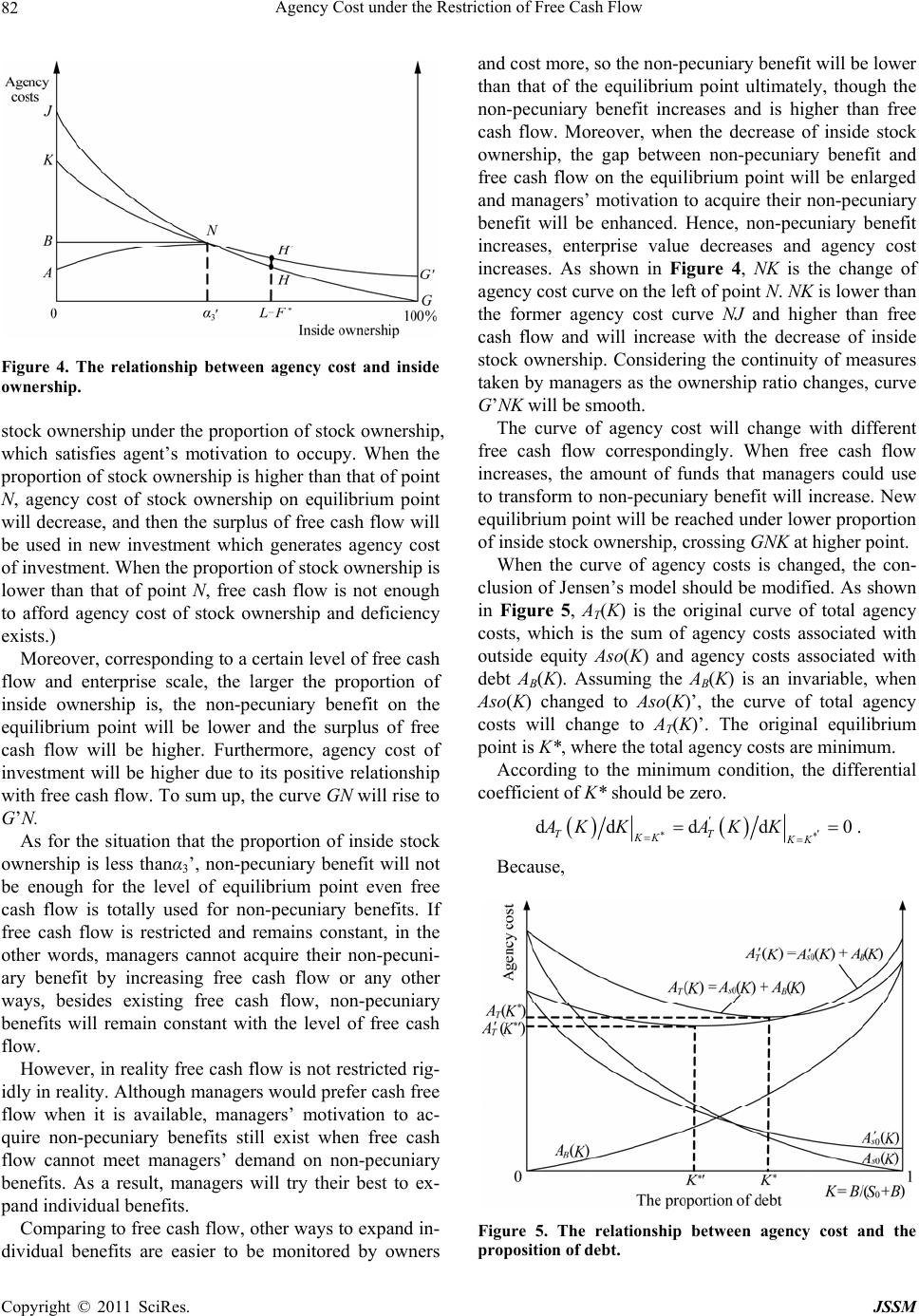 Agency Cost under the Restriction of Free Cash Flow 82 Figure 4. The relationship between agency cost and inside ownership. stock ownership under the proportion of stock ownership, which satisfies agent’s motivation to occupy. When the proportion of stock ownership is higher than that of point N, agency cost of stock ownership on equilibrium point will decrease, and then the surplus of free cash flow will be used in new investment which generates agency cost of investment. When the proportion of stock ownership is lower than that of point N, free cash flow is not enough to afford agency cost of stock ownership and deficiency exists.) Moreover, corresponding to a certain level of free cash flow and enterprise scale, the larger the proportion of inside ownership is, the non-pecuniary benefit on the equilibrium point will be lower and the surplus of free cash flow will be higher. Furthermore, agency cost of investment will be higher due to its positive relationship with free cash flow. To sum up, the curve GN will rise to G’N. As for the situation that the proportion of inside stock ownership is less thanα3’, non-pecuniary benefit will not be enough for the level of equilibrium point even free cash flow is totally used for non-pecuniary benefits. If free cash flow is restricted and remains constant, in the other words, managers cannot acquire their non-pecuni- ary benefit by increasing free cash flow or any other ways, besides existing free cash flow, non-pecuniary benefits will remain constant with the level of free cash flow. However, in reality free cash flow is not restricted rig- idly in reality. Although managers would prefer cash free flow when it is available, managers’ motivation to ac- quire non-pecuniary benefits still exist when free cash flow cannot meet managers’ demand on non-pecuniary benefits. As a result, managers will try their best to ex- pand individual benefits. Comparing to free cash flow, other ways to expand in- dividual benefits are easier to be monitored by owners and cost more, so the non-pecuniary benefit will be lower than that of the equilibrium point ultimately, though the non-pecuniary benefit increases and is higher than free cash flow. Moreover, when the decrease of inside stock ownership, the gap between non-pecuniary benefit and free cash flow on the equilibrium point will be enlarged and managers’ motivation to acquire their non-pecuniary benefit will be enhanced. Hence, non-pecuniary benefit increases, enterprise value decreases and agency cost increases. As shown in Figure 4, NK is the change of agency cost curve on the left of point N. NK is lower than the former agency cost curve NJ and higher than free cash flow and will increase with the decrease of inside stock ownership. Considering the continuity of measures taken by managers as the ownership ratio changes, curve G’NK will be smooth. The curve of agency cost will change with different free cash flow correspondingly. When free cash flow increases, the amount of funds that managers could use to transform to non-pecuniary benefit will increase. New equilibrium point will be reached under lower proportion of inside stock ownership, crossing GNK at higher point. When the curve of agency costs is changed, the con- clusion of Jensen’s model should be modified. As shown in Figure 5, AT(K) is the original curve of total agency costs, which is the sum of agency costs associated with outside equity Aso(K) and agency costs associated with debt AB(K). Assuming the AB(K) is an invariable, when Aso(K) changed to Aso(K)’, the curve of total agency costs will change to AT(K)’. The original equilibrium point is K*, where the total agency costs are minimum. According to the minimum condition, the differential coefficient of K* should be zero. dd dd TT KK KK AK KAK K 0 . Because, Figure 5. The relationship between agency cost and the proposition of debt. Copyright © 2011 SciRes. JSSM 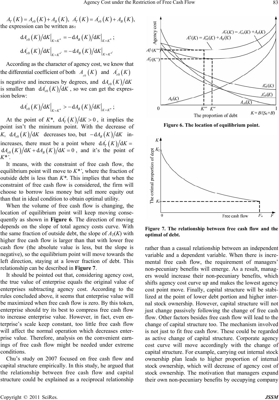 Agency Cost under the Restriction of Free Cash Flow 83 0Ts B KAKAK , 0Ts B KAKAK , the expression can be written as: 0 dd dd sB KK AK KAK K K ; 0 dd dd sB K KK AK KAK K According as the character of agency cost, we know that the differential coefficient of both 0s K and 0s K is negative and increases by degrees, and 0 dd s KK is smaller than 0 d sd KK , so we can get the expres- sion below: 0 dd dd sB K KK AK KAK K ; At the point of K*, dd T AKK 0, it implies the point isn’t the minimum point. With the decrease of K, 0 d sd KK decreases too, but d Bd KK in- increases, there must be a point where dd T KK 0 dddd sB AK KAK K0 , and it’s the point of K*’. It means, with the constraint of free cash flow, the equilibrium point will move to K*’, where the fraction of outside debt is less than K*. This implies that when the constraint of free cash flow is considered, the firm will choose to borrow less money but sell more equity out than that in ideal condition to obtain optimal utility. When the volume of free cash flow is changing, the location of equilibrium point will keep moving conse- quently as shown in Figure 6. The direction of moving depends on the slope of total agency costs curve. With the same fraction of outside debt, the slope of AT(K) with higher free cash flow is larger than that with lower free cash flow (the absolute value is less, but the slope is negative), so the equilibrium point will move towards the left direction, staying at a lower fraction of debt. This relationship can be described in Figure 7. It should be pointed out that, considering agency cost, the true value of enterprise equals the original value of enterprises subtracting agency cost. According to the rules concluded above, it seems that enterprise value will be maximized when free cash flow is zero. By this token, enterprise should try its best to compress free cash flow to increase enterprise value. However, in fact, even en- terprise’s scale keep constant, too little free cash flow will affect the normal operation which decreases enter- prise value. Therefore, analysis on the convenient earn- ings of free cash flow might be needed under extreme conditions. Chu’s study on 2007 focused on free cash flow and capital structure empirically. In this study, he argued that the relationship between free cash flow and capital structure could be explained as a reciprocal relationship Figure 6. The location of equilibrium point. Figure 7. The relationship between free cash flow and the optimal of debt. rather than a casual relationship between an independent variable and a dependent variable. When there is incre- mental free cash flow, the requirement of managers’ non-pecuniary benefits will emerge. As a result, manag- ers would increase their non-pecuniary benefits, which shifts agency cost curve up and makes the lowest agency cost point move. Finally, capital structure will be stabi- lized at the point of lower debt portion and higher inter- nal stock ownership. However, capital structure will not just change passively following the change of free cash flow. Other factors besides free cash flow will lead to the change of capital structure too. The mechanism involved is not just to fit free cash flow. These could be regarded as active change of capital structure. Corporate agency cost curve will move accordingly with the change of capital structure. For example, carrying out internal stock ownership plan leads to higher proportion of internal stock ownership, which will decrease of agency cost of stock ownership. The motivation that managers expand their own non-pecuniary benefits by occupying company Copyright © 2011 SciRes. JSSM 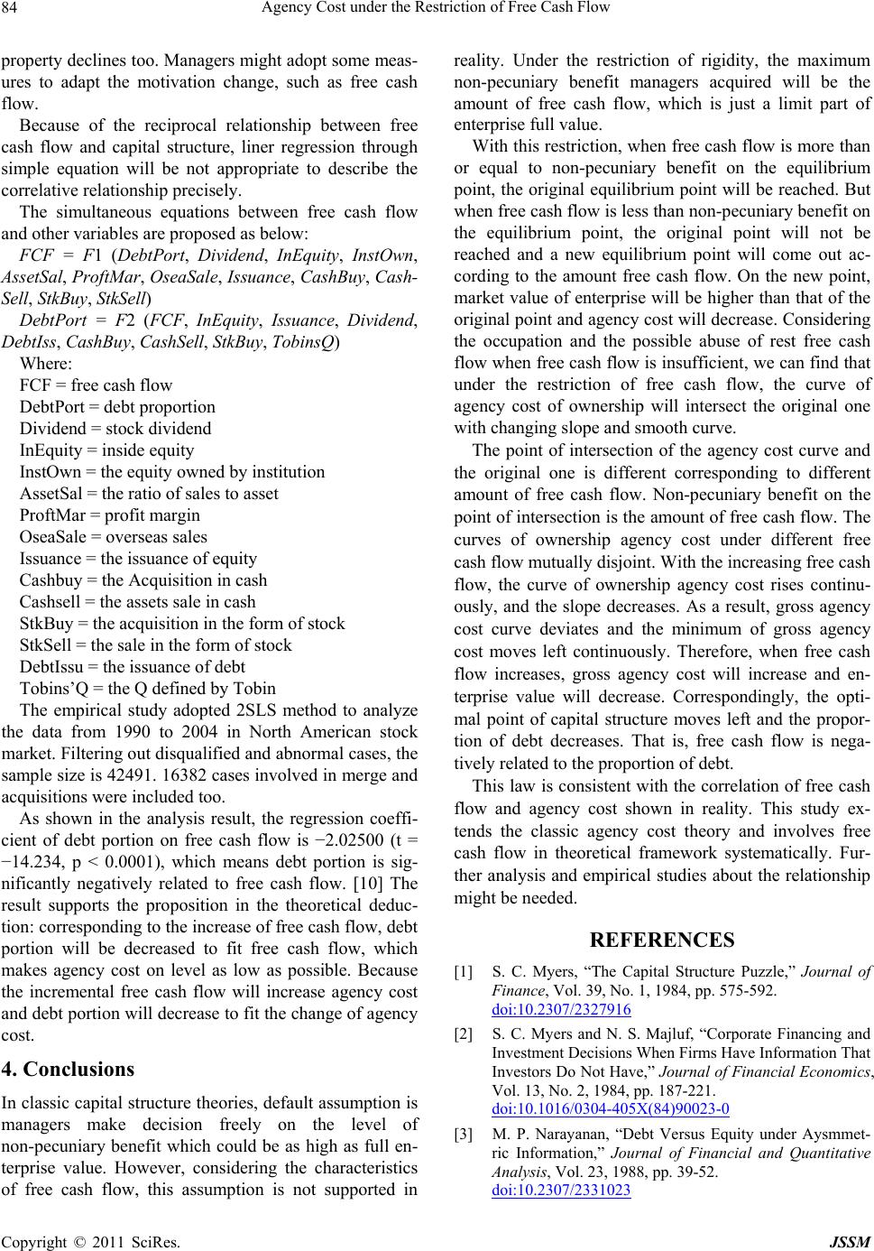 Agency Cost under the Restriction of Free Cash Flow 84 property declines too. Managers might adopt some meas- ures to adapt the motivation change, such as free cash flow. Because of the reciprocal relationship between free cash flow and capital structure, liner regression through simple equation will be not appropriate to describe the correlative relationship precisely. The simultaneous equations between free cash flow and other variables are proposed as below: FCF = F1 (DebtPort, Dividend, InEquity, InstOwn, AssetSal, ProftMar, OseaSale, Issuance, Ca shBu y, Cash- Sell, StkBuy, StkSell) DebtPort = F2 (FCF, InEquity, Issuance, Dividend, DebtIss, CashBuy , CashS e ll, StkBuy, TobinsQ) Where: FCF = free cash flow DebtPort = debt proportion Dividend = stock dividend InEquity = inside equity InstOwn = the equity owned by institution AssetSal = the ratio of sales to asset ProftMar = profit margin OseaSale = overseas sales Issuance = the issuance of equity Cashbuy = the Acquisition in cash Cashsell = the assets sale in cash StkBuy = the acquisition in the form of stock StkSell = the sale in the form of stock DebtIssu = the issuance of debt Tobins’Q = the Q defined by Tobin The empirical study adopted 2SLS method to analyze the data from 1990 to 2004 in North American stock market. Filtering out disqualified and abnormal cases, the sample size is 42491. 16382 cases involved in merge and acquisitions were included too. As shown in the analysis result, the regression coeffi- cient of debt portion on free cash flow is −2.02500 (t = −14.234, p < 0.0001), which means debt portion is sig- nificantly negatively related to free cash flow. [10] The result supports the proposition in the theoretical deduc- tion: corresponding to the increase of free cash flow, debt portion will be decreased to fit free cash flow, which makes agency cost on level as low as possible. Because the incremental free cash flow will increase agency cost and debt portion will decrease to fit the change of agency cost. 4. Conclusions In classic capital structure theories, default assumption is managers make decision freely on the level of non-pecuniary benefit which could be as high as full en- terprise value. However, considering the characteristics of free cash flow, this assumption is not supported in reality. Under the restriction of rigidity, the maximum non-pecuniary benefit managers acquired will be the amount of free cash flow, which is just a limit part of enterprise full value. With this restriction, when free cash flow is more than or equal to non-pecuniary benefit on the equilibrium point, the original equilibrium point will be reached. But when free cash flow is less than non-pecuniary benefit on the equilibrium point, the original point will not be reached and a new equilibrium point will come out ac- cording to the amount free cash flow. On the new point, market value of enterprise will be higher than that of the original point and agency cost will decrease. Considering the occupation and the possible abuse of rest free cash flow when free cash flow is insufficient, we can find that under the restriction of free cash flow, the curve of agency cost of ownership will intersect the original one with changing slope and smooth curve. The point of intersection of the agency cost curve and the original one is different corresponding to different amount of free cash flow. Non-pecuniary benefit on the point of intersection is the amount of free cash flow. The curves of ownership agency cost under different free cash flow mutually disjoint. With the increasing free cash flow, the curve of ownership agency cost rises continu- ously, and the slope decreases. As a result, gross agency cost curve deviates and the minimum of gross agency cost moves left continuously. Therefore, when free cash flow increases, gross agency cost will increase and en- terprise value will decrease. Correspondingly, the opti- mal point of capital structure moves left and the propor- tion of debt decreases. That is, free cash flow is nega- tively related to the proportion of debt. This law is consistent with the correlation of free cash flow and agency cost shown in reality. This study ex- tends the classic agency cost theory and involves free cash flow in theoretical framework systematically. Fur- ther analysis and empirical studies about the relationship might be needed. REFERENCES [1] S. C. Myers, “The Capital Structure Puzzle,” Journal of Finance, Vol. 39, No. 1, 1984, pp. 575-592. doi:10.2307/2327916 [2] S. C. Myers and N. S. Majluf, “Corporate Financing and Investment Decisions When Firms Have Information That Investors Do Not Have,” Journal of Financial Economics, Vol. 13, No. 2, 1984, pp. 187-221. doi:10.1016/0304-405X(84)90023-0 [3] M. P. Narayanan, “Debt Versus Equity under Aysmmet- ric Information,” Journal of Financial and Quantitative Analysis, Vol. 23, 1988, pp. 39-52. doi:10.2307/2331023 Copyright © 2011 SciRes. JSSM 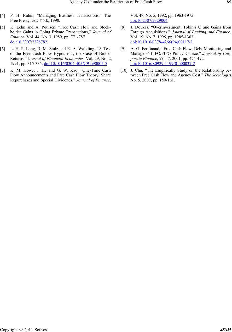 Agency Cost under the Restriction of Free Cash Flow Copyright © 2011 SciRes. JSSM 85 [4] P. H. Rubin, “Managing Business Transactions,” The Free Press, New York, 1990. [5] K. Lehn and A. Poulsen, “Free Cash Flow and Stock- holder Gains in Going Private Transactions,” Journal of Finance, Vol. 44, No. 3, 1989, pp. 771-787. doi:10.2307/2328782 [6] L. H. P. Lang, R. M. Stulz and R. A. Walkling, “A Test of the Free Cash Flow Hypothesis, the Case of Bidder Returns,” Journal of Financial Economics, Vol. 29, No. 2, 1991, pp. 315-335. doi:10.1016/0304-405X(91)90005-5 [7] K. M. Howe, J. He and G. W. Kao, “One-Time Cash Flow Announcements and Free Cash Flow Theory: Share Repurchases and Special Dividends,” Journal of Finance, Vol. 47, No. 5, 1992, pp. 1963-1975. doi:10.2307/2329004 [8] J. Doukas, “Overinvestment, Tobin’s Q and Gains from Foreign Acquisitions,” Journal of Banking and Finance, Vol. 19, No. 7, 1995, pp. 1285-1303. doi:10.1016/0378-4266(94)00117-L [9] A. G. Ferdinand, “Free Cash Flow, Debt-Monitoring and Managers’ LIFO/FIFO Policy Choice,” Journal of Cor- porate Finance, Vol. 7, 2001, pp. 475-492. doi:10.1016/S0929-1199(01)00037-2 [10] J. Chu, “The Empirically Study on the Relationship be- tween Free Cash Flow and Agency Cost,” The Sociologist, No. 5, 2007, pp. 159-161.
|