 Journal of Applied Mathematics and Physics, 2014, 2, 8-13 Published Online January 2014 (http://www.scirp.org/journal/jamp) http://dx.doi.org/10.4236/jamp.2014.21002 OPEN ACCESS JAMP Numerical Solution to Boundary Layer Problems over Moving Flat Plate in Non-Newtonian Media Gabriella Bognár, Zoltán Csáti Faculty of Mechanical Engineering and Informatics, University of Miskolc, Miskolc, Hungary Email: matvbg@uni-miskolc.hu Received September 2013 ABSTRACT Our aim is to investigate the solutions to the boundary layer problem of a power-law non-Newtonian fluid along an impermeable sheet moving with a constant velocity in an otherwise quiescent fluid environment. In the ab- sence of an exact solution in closed form, numerical solutions for the velocity distribution in the boundary layer for different power exponents will be presented. Our goal is to give an iterative transformation method for the determination of the skin friction parameter and the boundary layer thickness for different parameter values and the dependence of the skin friction parameter and the boundary layer thickness on the power exponent are examined. KEYWORDS Boundary Layer Problem; Non-Newtonian Fluid; Skin Friction Parameter; Iterative Transformation Method 1. Introduction The study of flow generated by a moving surface in an otherwise quiescent fluid plays a significant role in many material processing applications such as hot rolling, metal forming and continuous casting (see e.g., [1-3]). Boundary layer flow induced by the uniform motion of a continuous plate in a Newtonian fluid has been ana- lytically studied by Sakiadis [4] and experimentally applied by Tsou et al. [5]. A polymer sheet extruded conti- nuously from a die traveling between a feed roll and a wind-up roll was investigated by Sakiadis [4,6]. He pointed out that the known solutions for the boundary layer on surfaces of finite length are not applicable to the boundary layer on continuous surfaces. In the case of a moving sheet of finite length, the boundary layer grows in a direction opposite to the direction of motion of the sheet. Tsou et al. [5] showed in their analytical and experimental study that the obtained analytical results for the laminar velocity field are in excellent agreement with the measured data, therefore it validates that the mathe- matical model for boundary layer on a continuous moving surface describes a physically realizable flow. The problems of the boundary layer over a continuous surface moving in an otherwise quiescent fluid envi- ronment have attracted considerable attention (e.g., [1-3,5,7,8]). In this paper we use the power-law rheological model for the flow of a fluid over a sheet. In the absence of an exact solution in closed form, numerical solutions for the velocity distribution in the boundary layer for different power exponents will be presented, and the de- pendence of the skin friction parameter and the boundary layer thickness on the power exponent n are examined. 2. Mathematical Model 2.1. Boundary Layer Equations Consider the two-dimensional steady flow of a non-Newtonian fluid of density modeled by a power law fluid due to Ostwald-de Waele over a flat plate moving continuously with a constant velocity w U in an other- wise quiescent fluid medium [5]. The governing equations of motion and heat transfer for non-Newtonian flow neglecting pressure gradient, body forces can be described by the following equations [5]: 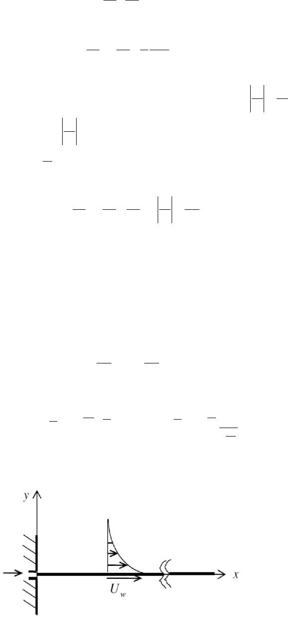 G. BOGNÁR, Z. CSÁTI OPEN ACCESS JAMP 9 0 uv xy ∂∂ ∂∂ , (1) and , (2) where , are the velocity components along and coordinates, respectively, is the temperature of the fluid in the boundary layer. Furthermore, we apply power-law relation between the shear stress and the shear rate, where 1n cu y µ − ∂ ∂ denotes the kinematic viscosity, the consistency index for non-Newtonian viscosity and . Here, n is called power-law index, that is for pseudoplastic, for Newtonian, and for dilatant fluids. Then, differential Equation (2) becomes [9] 1n c uu uu uv xyyy y µ − ∂ ∂∂∂∂ += ∂∂∂∂ ∂ . (3) The boundary conditions of the flow can be expressed as 0w u x,U=, , 0 y lim ux,y →∞ =. If a flat plate in surroundings at rest is moved with constant velocity the no-slip condition means that boundary layer exists close to the wall (see Figure 1). The moving plate emerges from the wall. This fixes the origin of the coordinate system and has an analog to the leading edge of a flat plate at zero incidence in a flow. Both permit only then a steady solution in a spatially fixed coordinate system. 2.2. Similarity Transformation Method The continuity Equation (1) is satisfied by introducing a stream function such that , . (4) The momentum equation can be transformed into the corresponding ordinary differential equation by the fol- lowing transformations ( ) 21 1 111 1 n nn n cw (x,y)Uxf( ) − ++ + =, ( ) 2 11 1 1 1 n n n cw n y U x ηµ − −+ + + =, where is the similarity variable and is the dimensionless stream function. Equation (3) with the transformed boundary conditions can be written as Figure 1. The physical model of the boundary layer on a continuously moving surface.  G. BOGNÁR, Z. CSÁTI OPEN ACCESS JAMP ( ) 1 10 1 n f fff n − ′ ′′ ′′′′ += + , (5) , , 0flim f η η →∞ ∞== , (6) where the prime denotes the differentiation with respect to the similarity variable . Equation (5) is called the generalized Sakiadis equation. The dimensionless velocity components have the form: , ( )( )( ) ( ) 1 1 n n wx U v x,yReff n ηη η + ′ = − + , and , where 2nn x ReUx/ K ρ − ∞ = is the local Reynolds number. Since the pioneering work by Acrivos [10], different approaches have been investigated for in the case of non-Newtonian fluids. It has a physical meaning: drag force or force due to skin friction. It is a fluid dy- namic resistive force which is a consequence of the fluid and the pressure distribution on the surface of the ob- ject. The skin friction parameter originates from the non-dimensional drag coefficient ()( )( ) 11 1 1 1 00 n n n n D CnRef ''f '' − + + − = + , and it is involved in the wall shear stress ()( )( ) 1 311 00 nn nn w wn KU xf ''f '' x ρ τ +− = . The boundary value problem (5), (6) is defined on a semi-infinite interval [11]. For Newtonian fluids ( ), Equation (5) is the well-known Blasius equation: . (7) Blasius [12] solved Equation (7) subject to boundary conditions f′=, f=, 1flim f η η →∞ ∞== (8) by patching a power series to an approximation at some finite value of . An iterative transformation method was introduced for (7), (8) by Töpfer for the determination of (see [13]). Equation (5) with (8) is called the generalized Blasius problem [12]. For non-Newtonian fluids on steady sur- faces, the boundary value problem (5), (6) has been investigated in [14,15] and for Newtonian fluid in [16,17]. The aim of this paper is to give a method for the determination of the skin friction parameter and the boundary layer thickness for different parameter values n. 3. Iterative Transformation Method In this section an iterative transformation method (ITM) is developed to solve the boundary value problem (5), (6). Solving this problem, we have to deal with a practically unsuited condition at infinity. To tackle this com- putational difficulty, we apply the so-called scaling concept. Non-iterative and iterative transformation methods for boundary value problems have been introduced by Fazio [18]. The idea behind the present method is to consider the “partial” invariance of (5), (6) with respect to a scaling transformation in the sense that the differential equation and one of the boundary conditions at 0 are invariant, while the other two boundary conditions are not invariant. Therefore, we modify the problem by introducing a numerical parameter h. Now, Equation (5) is to be solved with boundary conditions 0 0,f= ()( ) 1, p f 'limf 'h η η →∞ ∞= =− where we involve h, to ensure the invariance of the extended scaling group. We introduce the following transformations to convert the boundary value problem to an initial value problem,  G. BOGNÁR, Z. CSÁTI OPEN ACCESS JAMP 11 where the following scaling transformation is applied and 0f'' σ = − is denoted: . Equation (5) is scaling invariant if 2 12 . (9) Then, one gets ( ) 1 10 1 n g ggg n − ′ ′′ ′′′′ += + . (10) The appropriate boundary conditions can be determined from the proper derivatives of f: (11) ( )( ) ( ) pp * fh gh βα γ −− (12) ( )( ) ( ) 11 pp * hf hg βα γ λλ − − ′′ ∞=− ⇒∞=− (13) . (14) We can observe from Equation (11) that the first boundary condition in (6) is scaling invariant. The other two boundary conditions are not invariant. Now, let and . From (9), (12) and (14) we get the following expressions for the scaling parameters: , , 11 3 n p γ + = −. (15) Utilizing the boundary condition prescribed at infinity, from (13) we gain a formula for the sought value of 0f σ ′′ = −: ( ) ( ) 3 1 *p n gh σ −+ ′ = ∞+ (16) During the calculating process, p is freely chosen. Now, we can write the initial values in their final forms: , , . (17) The initial value problem (10), (17) is solved with the so-called iterative transformation method. Its steps are enumerated below: 1) A numerical parameter h is applied so that two boundary conditions remain invariant. 2) By starting with a suitable value of , a root finder algorithm is used to define a sequence for . After each iteration the group parameter is obtained by solving the IVP numerically. The se- quence is defined by . 3) An adequate termination criteria must be used to verify whether as . 4) The solution of the original problem can be received by rescaling to . 4. Results The nonlinear ordinary differential Equation (10) with the boundary conditions in (17) was solved for some val- ues of the power-law index n by MATLAB. The built-in ode113, a variable order Adams-Bashforth-Moulton solver was used with default accuracy and adaptivity parameters and was determined when the local error was less than . As for the root finder algorithm, we programmed the bisection method because of safety considerations. We may remark that if is demanded to decrease monotonically, then is negative for every possible . Therefore choosing a positive number for , h never reaches 1 which is the case for [19]. Numerical results for function values 0f'' are shown below in Table 1. For n = 1 we reproduced the result achieved by Fazio. Figure 2 illustrates the function, which is  G. BOGNÁR, Z. CSÁTI OPEN ACCESS JAMP Table 1. Numerical results for . n 0.96 0.97 0.98 0.99 1 1.1 1.2 fʺ)0( −0.443438 −0.443438 −0.443286 −0.443193 −0.443726 −0.436611 −0.409834 n 1.3 1.4 1.42 1.45 1.48 1.49 1.5 fʺ)0( −0.361843 −0.282487 −0.259809 −0.217169 −0.154069 −0.123517 −0.081410 Figure 2. Similarity velocity profiles for power-law non-Newtonian fluid. proportional to the non-dimensional velocity component, for different power law indices n. Acknowledgements The research work presented in this paper is based on the results achieved within the TÁMOP-4.2.1.B-10/2/ KONV-2010-0001 project and carried out as part of the TÁMOP-4.1.1.C-12/1/KONV-2012-0002 “Cooperation between higher education, research institutes and automotive industry” project in the framework of the New Széchenyi Plan. The realization of this project is supported by the Hungarian Government, by the European Un- ion, and co-financed by the European Social Fund. REFERENCES [1] T. Altan, S. Oh and H. Gegel, “Metal Forming Fundamentals and Applications,” American Society of Metals, Metals Park, 1979. [2] E. G. Fisher, “Extrusion of Plastics,” John Wiley, New York, 1976. [3] Z. Tadmor and I. Klein, “Engineering Principles of Plasticating Extrusion, Polymer Science and Engineering Series,” Van Nor- strand Reinhold, New York, 1970. [4] B. C. Sakiadis, “Boundary Layer Behavior on Continuous Solid Surfaces: I. Boundary Layer Equations for Two-Dimensional and Axisymmetric Flow,” AIChE Journal, Vol. 7, 1961, pp. 26-28. http://dx.doi.org/10.1002/aic.690070108 [5] F. Tsou, E. M. Sparrow and R. Goldstein, “Flow and Heat Transfer in the Boundary Layer on a Continuous Moving Surface,”  G. BOGNÁR, Z. CSÁTI OPEN ACCESS JAMP 13 International Journal of Heat and Mass Transfer, Vol. 10, 1967, pp. 219-235. http://dx.doi.org/10.1016/0017-9310(67)90100-7 [6] B. C. Sakiadis, “Boundary Layer Behavior on Continuous Solid Surfaces. II: The Boundary Layer on a Continuous Flat Surface, AIChE Journal, Vol. 7, 1961, pp. 221-225. http://dx.doi.org/10.1002/aic.690070211 [7] M. Y. Hussaini, W. D. Lakin and A. Nachman , “On Similarity Solutions of a Boundary Layer Problem with an Upstream Mov- ing Wall,” SIAM Journal on Applied Mathematics, Vol. 47, 1987, pp. 699-709. http://dx.doi.org/10.1137/0147048 [8] A. Nachman and A. J. Callegari, “A Nonlinear Singular Boundary Value Problem in the Theory of Pseudoplastic Fluids,” SIAM Journal on Applied Mathematics, Vol. 38, 1980, pp. 275-281. http://dx.doi.org/10.1137/0138024 [9] M. Benlahsen, M. Guedda and R. Kersne r, “The Generalized Blasius Equation Revisited,” Mathematical and Computer Model- ling, Vol. 47, 2008, pp. 1063-1076. http://dx.doi.org/10.1016/j.mcm.2007.06.019 [10] A. Acrivos, M. J. Shah and E. E. Peterson, “Momentum and Heat Transfer in Laminar Boundary Flow of Non-Newtonian Flu- ids past External Surfaces,” AIChE Journal, Vol. 6, 1960, pp. 312-317. http://dx.doi.org/10.1002/aic.690060227 [11] H. Weyl, “On the Differential Equations of the Simplest Boundary-Layer Problems,” Annals of Mathematics, Vol. 43, 1942, pp. 381-407. http://dx.doi.org/10.2307/1968875 [12] H. Blasius, “Grenzschichten in Flussigkeiten mit Kleiner Reibung,” Zeitschrift für angewandte Mathematik und Physik, Vol. 56, 1908, pp. 1-37. [13] K. Töpfer, “Bemerkung zu dem Aufsatz von H. Blasius: Grenzschichten in Flüssigkeiten mit kleiner Reibung,” Zeitschrift für angewandte Mathematik und Physik, Vol. 60, 1912, pp. 397-398. [14] G. Bognár, “Similarity Solutions of Boundary Layer Flow for Non-Newtonian Fluids,” International Journal of Nonlinear Sciences and Numerical Simulation, Vol. 10, 2010, pp. 1555-1566. http://dx.doi.org/10.1515/IJNSNS.2009.10.11-12.1555 [15] G. Bognár, “Iterative Transformation Method for the Boundary Layer Problems of Non-Newtonian Fluid Flows along Moving Surfaces, to Appear.” [16] A. J. Callegari and M. B. Friedman, “An Analytical Solution of a Nonlinear, Singular Boundary Value Problem in the Theory of Viscous Flows,” Journal of Mathematical Analysis and Applications, Vol. 21, 1968, pp. 510-529. http://dx.doi.org/10.1016/0022-247X(68)90260-6 [17] M. Y. Hussaini and W. D. Lakin, “Existence and Nonuniqueness of Similarity Solutions of a Boundary-Layer Problem,” Quar- terly Journal of Mechanics & Applied Mathematics, Vol. 39, 1986, pp. 177-191. http://dx.doi.org/10.1093/qjmam/39.1.15 [18] R. Fazio, “A Novel Approach to the Numerical Solution of Boundary Value Problems on Infinite Intervals,” Journal on Nume- rical Analysis, Vol. 33, 1996, pp. 1473-1483. http://dx.doi.org/10.1137/S0036142993252042 [19] R. Fazio, “The Iterative Transformation Method for the Sakiadis Problem,” 2011. http://mat521.unime.it/fazio/preprints/Sakiadis.pdf
|