 Journal of Mathematical Finance, 2014, 4, 1-9 Published Online January 2014 (http://www.scirp.org/journal/jmf) http://dx.doi.org/10.4236/jmf.2014.41001 OPEN ACCESS JMF Evaluation of Geome tric Asian Power Options under Fractional Brownian Motion Zhijuan Mao1, Zhian Liang2 1School of Finance, Shanghai University of Finance and Economics, Shanghai, China 2Department of Applied Mathematics, Shanghai University of Finance and Economics, Shanghai, China Email: zmao86@gmail.com Received October 12, 2013; revised November 21, 2013; accepted December 6, 2013 Copyright © 2014 Zhijuan Mao, Zhian Liang. This is an open access article distributed under the Creative Commons Attribution License, which permits unrestricted use, distribution, and reproduction in any medium, provided the original work is properly cited. In accordance of the Creative Commons Attribution License all Copyrights © 2014 are reserved for SCIRP and the owner of the intellectual property Zhijuan Mao, Zhian Liang. All Copyright © 2014 are guarded by law and by SCIRP as a guardian. ABSTRACT Modern option pricing techniques are often considered among the most mathematical complex of all applied areas of financial mathematics. In particular, the fractional Brownian motion is proper to model the stock dy- namics for its long-range dependence. In this paper, we evaluate the price of geometric Asian options under frac- tional Brownian motion framework. Furthermore, the options are generalized to those with the added feature whose payoff is a power function. Based on the equivalent martingale theory, a closed form solution has been derived under the risk neutral probability. KEYWORDS Fractional Brownian Motion; Geome tric Asian Options; Closed-Form Solution; Risk-Free Rate 1. Introduction Estimating option pricing is a central topic in financial mathematics. A call (put) option is a contract which gives the holder the right but not the obligation, to buy (sell) a risky asset at a certain date with a predetermined price (called strike price). In terms of the execution time, options can be classified into three types: American options whose owner can choose to exercise at any time up to and including the expiration; Bermudan options which permit early exercise but only on a contractually specified finite set of dates; European options which can only be exercised at the expiration date. The European calls and puts, which are with maturity T and strike price K, are often called vanilla options. And their payoffs at maturity, i.e., ST K and KST , respectively, depend only on the spot value of the underlying asset. On the other hand, there exist several kinds of exotic options such as Asian options, look-back options and knock-out options. In 1987, Asian options were first introduced at a branch of an American bank in Tokyo, Japan. For an Asian option, its payoff is determined by the average value over some predetermined time interval. One advantage is that it can reduce the risk of market manipulation of the underlying instrument at maturity. Moreover, they offer better hedging possibilities for firms with a stream of exposures. Another benefit is that they are useful in pro- tecting the owner from sudden short lasting price changes in the market, for example, due to order imbalances [1]. Because of the averaging property, Asian options reduce the volatility inherent in the option. And therefore, Asian options are usually cheaper comparing with its European counterparts. Asian options have numerous permutations, such as fixed and floating strike price options. The payoff of fixed strike options is TK , KAT for a call and put option, respectively, where K denotes the strike price and T is the average price of the underlying asset. For floating strike price options, the payoff takes the following form: ST AT and AT ST for a call and put option, respectively. In terms of the average price T, Asian options can be classified into two categories: arithmetic average  Z. J. MAO, Z. LIANG 2 Asians and geometric average Asians, and both these forms can be averaged on a weighted average basis. For the continuous case, arithmetic average is obtained by 0 1d. T TSt T t And the geometric average is given by 0 1ln d e. (1) TSt t T AT For the discrete case, we just need to change the integral into summation. In this sequel, we just consider the case of continuous geometric average with fixed strike price and leave the discrete case for readers. An Asian option (also called average value option) is an important class of path-dependent options and its pricing has aroused much attention. The path integral formalism was created by Richard Feynman in quantum physics [2]. Norbert Wiener used this type of integral in his research of Brownian motion [3]. And Jan Dash first introduced this type of path integral into finance, who developed empirical studies related to the Black-Scholes- Merton model and the one-factor term structure constrained model. Till now, there is no known closed form so- lution for the arithmetic type, for it is difficult to analytically evaluate the sum of the related log-normal random variables. Feynman and Kleinert showed that by the method of the path integral, the problem for geometric av- erage can be solved via the effective classical potential [4]. In 1990, Kemna and Vorst discussed the pricing of arithmetic Asian options with MCMC method and proposed Turnbull and Wakeman formula for pricing Arith- metic average option under continuous case. Furthermore, they derived an analytic solution for a geometric av- erage option by changing the diffusion term [5]. In 1995, Rogers and Shi solved the pricing problem with a PDE approach [6]. On the other hand, the introduction of fractional Brownian motion (FBM) should date back to the develop- ment of the option pricing theory. In 1900, Bachelier, the father of option pricing theory, first developed arith- metic Brownian motion to model the dynamics of underlying asset [7]. In 1973, F. Black and M. Scholes intro- duced the Black-Scholes-Merton (BSM) model, which assumed that the stock process followed a geometric Brownian motion. And they derived the well-known BS formula [8]. But empirical studies indicate that the log-returns are usually not normal and show the dependence structure. Additionally, it also reveals that the stock price usually has some properties such as “fat tail”, “self-similarity”, “long-range dependence” [9]. This reveals the disparity between the model and the market. In 1940, Kolmogorov first introduced the fractional Brownian motion within a Hilbert space, where it was called Wiener Helix. Yaglom studied this process and discussed its moment properties [10]. Further studies have discovered that fractional Brownian motion can be used to model such situations as 1) The widths of consecutive annual rings of a tree; 2) The temperature at a specific place as a function of time; 3) The level of water in a river as a function of time; 4) The characters of solar activity as a function of time; 5) The values of the log returns of a stock; 6) Financial turbulence, i.e., the empirical volatility of a stock, and other turbulence phenomena; 7) The prices of electricity in a liberated electricity market. In 1968, Mandelbrot and Van Ness provided a stochastic integral representation of this process: If 0 < H < 1, the fractional Brownian motion with Hurst index H is a continuous Gaussian process, , and 00 HH BttRB with mean zero and covariance: 22 2 1., 2 HH H H tsosCts tv Obviously, H t coincides with B(t), the standard Brownian motion, when 12H. In 2008, Ciprian Necula obtained an explicit fractional BS formula by using Fourier transform [11]. Mandelbrot and Taylor pro- posed that the stock market should take on the character of fractional Brownian motion [12]. Then Peters intro- duced fractional Brownian motion to model the dynamics of stock price [13]. After this, many scholars have made outstanding contributions on this topic. In 2000, Duncan et al., Hu and Oksendal developed the fractional OPEN ACCESS JMF  Z. J. MAO, Z. LIANG 3 BS formula by using Wick-product [14]. And the systematic option pricing theory under fractional Brownian motion framework has been presented by Hu et al. in [15]. The paper is organized as follows. In Section 2, we further give a simple description of fractional Brownian motion framework and review some existing results of power options. Next, the pricing model of Geometric Asian power options has been presented in Section 3. Moreover, closed form solution and call-put parity are also derived. The conclusion remarks and some open problems are discussed in the final part. 2. Preliminary In general, one can rely on the numerical methods for pricing arithmetic Asian options in Levy models [16]. While geometric averaging options within Levy models can be priced analytically. Since its statistical property can be obtained from the assumption that the stock process follows a log-normal distribution. Kemna and Vorst [5] derived an analytic formula for Asian options of this kind as below. Lemma 2.1 For a geometric average Asian call option, its payoff is given as TK , where K is the strike price and 0 0 1ln d e T TStt TT AT with 0,TT being the final time interval over which the average value of the stock is calculated. Then T is log-normally distributed and thus the value of the option at time is as following: 0 T 200 11 26 00 012 ,e e rTT rT T NN CSTTSTF dKF d , where 02 0 12 0 11 ln 1 26 and . 3 13 ST rTT K dd TT 10 dTT In the FBM framework, stock is assumed to be the underlying asset and denoted by S(t) for simplicity. Then the price process can be modeled by the following PDE: ddd H St tBt St , (2) where is the spot price of the underlying security at time t, St , are both constant, H t being the standard FBM. Under risk neutral probability, (2) turns into the following form: ddd H St rtB t St , (3) where r is the risk-free rate and H t is the FBM under the new measure. The corresponding fractional BS formula was developed in [13,17]. For a European call option, its price process ,CSt t satisfies the fol- lowing PDE: 2 222 1 20. HCCC HS trSrC St S Solving the above PDE obtains the pricing formula: 12 0,00, NN CSSFdKF d where N F denotes the cumulative distribution function of standard normal distribution with 2 2 12 0 ln 2,. H 1 H SrT T K dd T dT Furthermore, Biagini and Oksendal etc. extended the model by assuming that the risk-free rate and dividend rate are non-random functions [15]. Then the option pricing formula under FBM framework is given as below: OPEN ACCESS JMF  Z. J. MAO, Z. LIANG 4 Lemma 2.2 Suppose the dynamics of asset price follows PDE (3) under the risk neutral probability. If the risk-free rate rt and dividend rate qt are non-random functions and the payoff function at maturity , STT is bounded, then the price of a European option ,VSt t satisfies the following: 222 22 2 1 d d22 1 ,ee ed 2π THH HH Tt t xrsqssT tT tx rs s VSt tf Stx . Recently, kinds of derivatives have been introduced to satisfy the need of market. Power options, one kind of the newly developed options, have aroused more and more attention. They are used to change the return struc- ture and also possess more flexibility comparing with vanilla options. Power options can be seen as instruments of risk management and getting higher return, thus attracting more and more application. For a European power call, there exist two types in terms of different payoff functions: if , if nn n ST KSTK fST TST KSTK , where n is a positive number. In 2005, Y. Wang et al. [18] derived an explicit formula of European power options. And Y. Xiao et al. [19] studied some properties of power options under Brownian motion framework. D. In 2006, Y. Wang et al. [20] generalized the model to Geometric Asian power options and obtained the solution under continuous case. In this paper, we further extend the underlying asset follows a fractional Brownian motion. Zhao [21] and S. Zhou [22] considered the European power options under FBM framework and deduced the pricing formula and call- put parity as well. In this paper, we consider the Asian power options under FBM framework. Correspondingly, for an Asian power call option with fixed strike price K and maturity T, there exist two types of payoff functions: if (4) , if (5) nn n AT KATK fATT AT KATK , where T is defined as (1). We discuss the case of (4), since the results for the other type can be obtained by the same procedure. 3. Pricing Model 3.1. General Hypotheses The general assumptions in this model are as below: A1 The dynamics of underlying asset follows fractional Brownian motion. A2 The risk-free rate r(t) is non-random function. A3 There are no transaction costs or taxes in buying or selling stocks, options, i.e., the market is frictionless. A4 Dividends are paid on the underlying stock during the option life with the rate of q(t). A5 The option can only be exercised at maturity. A6 The market does not admit arbitrage. 3.2. Pricing Framework with Constant Risk Free Rate and Dividend Rate Before coming to the case of non-random risk-free rate, we first consider the case that the risk-free rate and dividend rate are both constant. Let for simplicity. Under above assumptions, the dynamics of stock price process (3) takes the following form under risk neutral measure: 0t ddd H St rqtBt St , where r, q are the risk-free rate and dividend rate, respectively, H t being the FBM under risk-neutral probability. Then the stock price process can be derived OPEN ACCESS JMF  Z. J. MAO, Z. LIANG 5 22 1 0exp . 2 HH StSr qttBt It implies that is log-normally distributed with St 22 22 1 lnln 0, 2 HH StNSr qttt under risk neutral measure. First, we derive the closed form solution for Geometric Asian options with fixed strike price. Since its payoff at maturity is TK , the following theorem is derived: Theorem 3.1 Suppose the dynamics of underlying asset follows PDE (3) under risk neutral probability. If the risk free rate rt and dividend rate qt are constant, then a Geometric Asian call option at time 0t is priced as below: 22 11 24211 12 0, 0ee, H rqT T HH rT NN CSTSF dKF d where 22 212 011 ln 2221 and . 21 21 H H H SrqT T KH T dd TH H d (6) Proof of Theorem 3.1 Define 0 1ln d T GTStt T and exp . TGT From the definition, GT is normally distributed with mean and variance 2 , which are calculated explicitly as below. 0 22 00 22 1ln d 11 ln 0dd 2 11 ln 02221 T TT H EGTESt t T Srqttt TT SrqT T H t and 2 2 2 200 2 200 22 22 2 1dd 1dd 2 1 21 TT HH TT H HHH VarG TEG T EB tBt ts T ts T T H t , where denotes the expectation under risk neutral probability. Consequently, we can conclude that T is log-normally distributed, i.e., 2 ln, .AT GT N .K For a geometric Asian option, its payoff at maturity is Hence under the risk neutral measure, the value of a call option is: expAT KGT 2 2 2 1 0, eeeed, 2π x rTrTx D CSTE ATKKx where ::e x. xAT KxK And simple computations lead to that: OPEN ACCESS JMF 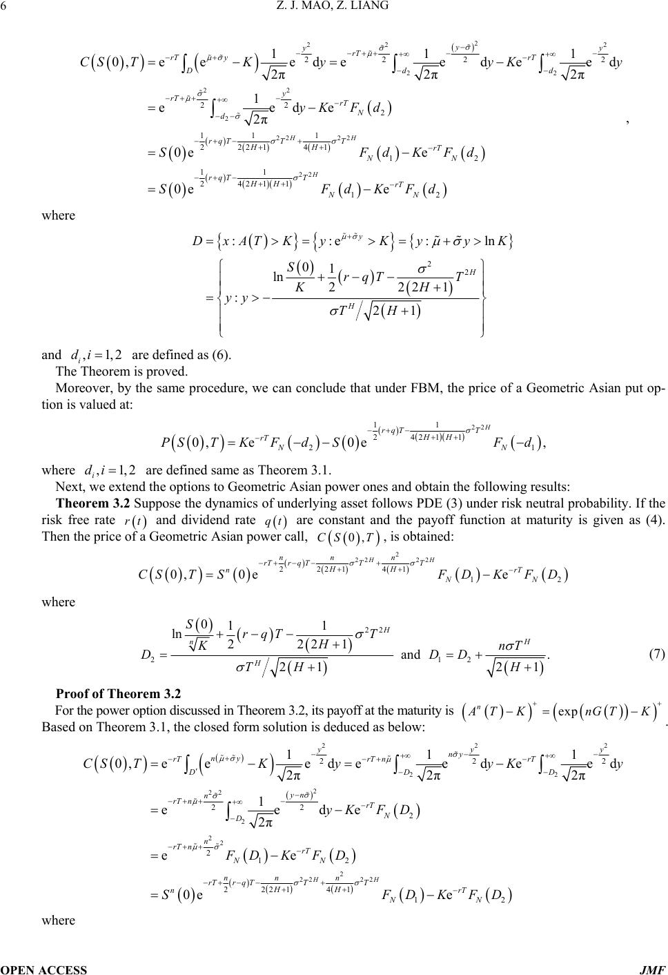 Z. J. MAO, Z. LIANG 6 2 22 22 22 2 22 22 22 22 2 22 2 11 1 2221 41 12 11 24211 11 eeed eedeed 2π2π2π 1 eede 2π 0e e 0e 0, HH y y y rT rT yrT Dd y rT rT N d rqT TT HH rT NN rqT T HH 2 2 1 d yyK yK Fd SFdKFd S CS T 12 e H rT NN FdK Fd y , where 2 2 ::e: 0 ln 2221 : 21 1 y H H DxATKyKy yK SrqT T KH yy TH ln and are defined as (6). ,1,2 i di The Theorem is proved. Moreover, by the same procedure, we can conclude that under FBM, the price of a Geometric Asian put op- tion is valued at: 22 11 24211 21 0, e0e, H rqT T HH rT NN PST K FdSFd where are defined same as Theorem 3.1. ,1,2 i di Next, we extend the options to Geometric Asian power ones and obtain the following results: Theorem 3.2 Suppose the dynamics of underlying asset follows PDE (3) under risk neutral probability. If the risk free rate rt and dividend rate qt are constant and the payoff function at maturity is given as (4). Then the price of a Geometric Asian power call, 0,CST , is obtained: 2 22 22 2221 41 12 0, 0ee HH nn n rTrq TTT HH nrT NN CSTSF DKF D where 22 212 011 ln 2221 and . 21 21 H H n H SrqT T H Kn DD TH H T D (7) Proof of Theorem 3.2 For the power option discussed in Theorem 3.2, its payoff at the maturity is exp n AT KnGTK . Based on Theorem 3.1, the closed form solution is deduced as below: 22 22 2 22 2 22 2 2222 22 22 2 2 12 2221 41 11 0,eee deedee d 2π2π2π 1 eede 2π ee 0e HH yy ny ny rTrT nrT DD yn n rT nrT N D n rT nrT NN nn n rTrqTTT HH n CSTKyy Ky yK FD FD K FD SF 12 erT NN DKFD 2 2 1 y D where OPEN ACCESS JMF  Z. J. MAO, Z. LIANG 7 2 2 ::e: 0 ln 2221 : 2 1 1 nny n H n H DxATKyKyy K SrqT T H K yy TH ln and are defined as (7). ,1,2 i Di The proof is complete. Furthermore, similar procedure obtains the price of the corresponding put option: 2 22 22 2221 41 2 1 0, e0e, HH nn n rTrq TTT HH rT n PSTKN DSN D where are defined same as Theorem 3.2. ,1,2 i Di 3.3. Generalized Pricing Framework Finally we consider the case that the risk-free rate and dividend rate are non-random functions. Under the risk neutral measure, the dynamics of stock price is obtained 22 0 1 0exp d. 2 tHH StSrsqsstBt Thus we obtain that is log-normally distributed and St 22 22 0 1 lnln 0d,. 2 tHH StNSrs qsstt Consider that T is defined as (1), and we denote 2 ln, .AT N Simple computations lead to 22 00 222 11 ln0dd, 22 1 1. 21 Tt H H STrsq HT T H sst Furthermore, the desired formula of option price can be derived as below: 2 0 22 00 22 2 22 00 2 22 00 d2 dd 22 dd 22 2 dd 2 12 1 0,eee d 2π 11 eedeed 2π2π 1 eede 2π ee 0e T TT TT TT y rs sny D yy ny rs snrs s DD yn n rss nrss N D n rss nrs s NN n CS TKy yK y yK Fd FD KFD S 22 222 000 0 ddd d 22 141 12 e, HH TTt T nnTnT rs srsqsstrss THH NN FD KFD where 22 0 122 0 011 lnd d 22 1and . 21 21 Tt H H n H STrsqsst HT Kn DD THH T D (8) As for the geometric Asian power put option, its price takes the following form: OPEN ACCESS JMF 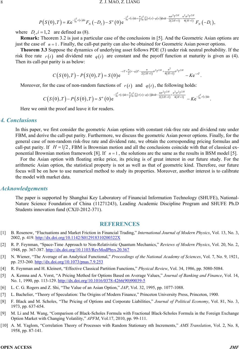 Z. J. MAO, Z. LIANG 8 22 222 000 0 ddd d22 141 2 1 0, e0e, HH TTt TnnTnT rs srsqsst rs sTHH n N N PSTKF D SF D where are defined as (8). ,1,2 i Di Remark: Theorem 3.2 is just a particular case of the conclusions in [5]. And the Geometric Asian options are just the case of . Finally, the call-put parity can also be obtained for Geometric Asian power options. 1n Theorem 3.3 Suppose the dynamics of underlying asset follows PDE (3) under risk neutral probability. If the risk free rate rt and dividend rate qt are constant and the payoff function at maturity is given as (4). Then its call-put parity is as below: 2 22 22 2221 41 0,0,0ee . HH nnn rTrq TTT HH rT CS TPS TSK Moreover, for the case of non-random functions of rt and qt, the following holds: 22 222 0000 ddd d 22 141 0,0,0ee . HH TTt T nnTnT rs srsqsstrss THH n CS TPS TSK Here we omit the proof and leave it for readers. 4. Conclusions In this paper, we first consider the geometric Asian options with constant risk-free rate and dividend rate under FBM, and derive the call-put parity. Furthermore, we discuss the geometric Asian power options. Finally, for the general case of non-random risk-free rate and dividend rate, we obtain the corresponding pricing formulas and call-put parity. If 12H, FBM is Brownian motion and all the conclusions coincide with that of classical ex- ponential Brownian motion framework [8]. If 1n , the solutions are the same as the results in BSM model [5]. For the Asian option with floating strike price, its pricing is of great interest in our future study. For the arithmetic Asian option, the statistical property is not as well as that of geometric kind. Therefore, our future focus will be on how to use numerical method to study its properties. Moreover, another interest is to calibrate the model with market data. Acknowledgements The paper is supported by Shanghai Key Laboratory of Financial Information Technology (SHUFE), National- Nature Science Foundation of China (11271243), Leading Academic Discipline Program and SHUFE Ph.D Students innovation fund (CXJJ-2012-371). REFERENCES [1] B. Rosenow, “Fluctuations and Market Friction in Financial Trading,” International Journal of Modern Phy s i cs, Vol. 13, No. 3, 2002, p. 419. http://dx.doi.org/10.1142/S012918310200322X [2] R. P. Feynman, “Space-Time Approach to Non-Relativistic Quantum Mechanics,” Reviews of Modern Physics, Vol. 20, No. 2, 1948, pp. 367-387. http://dx.doi.org/10.1103/RevModPhys.20.367 [3] N. Wiener, “The Average of an Analytical Functional,” Proceedings of the National Academy of Sciences, Vol. 7, No. 9, 1921, pp. 253-260. http://dx.doi.org/10.1073/pnas.7.9.253 [4] R. Feynman and H. Kleinert, “Effective Classical Partition Functions,” Physical Review, Vol. 34, 1986, pp. 5080-5084. [5] A. Kemna and A. Vorst, “A Pricing Method for Options Based on Average Values,” Journal of Banking and Finance, Vol. 14, No. 1, 1990, pp. 113-129. http://dx.doi.org/10.1016/0378-4266(90)90039-5 [6] L. C. G. Rogers and Z. Shi, “The Value of an Asian Option,” JAP, Vol. 32, 1995, pp. 1077-1088. [7] L. Bachelier, “Theory of Speculation: The Origins of Modern Finance,” Princeton University Press, Princeton, 1900. [8] F. Black and M. Scholes, “The Pricing of Options and Corporate Liabilities,” Journal of Political Economy, Vol. 81, No. 3, 1973, pp. 637-654. [9] M. Li and M. Wang, “Comparison of Black-Scholes Formula with Fractional Black-Scholes Formula in the Foreign Exchange Option Market with Changing Volatility,” APFM, Vol.17, 2010, pp. 99-111. [10] A. M. Yaglom, “Correlation Theory of Processes with Random Stationary nth Increments,” AMS Translation, Vol. 2, No. 8, 1958, pp. 87-141. OPEN ACCESS JMF 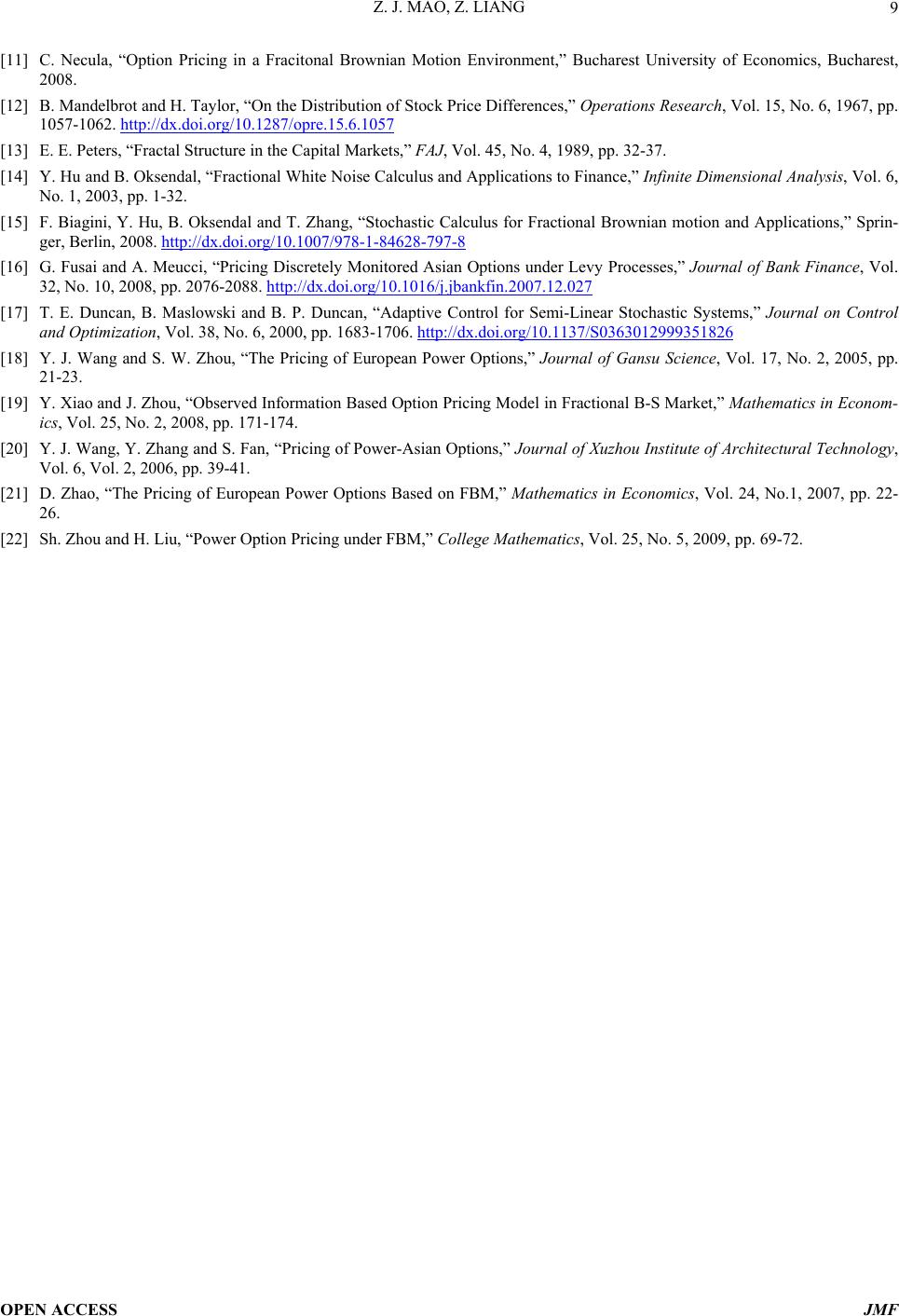 Z. J. MAO, Z. LIANG OPEN ACCESS JMF 9 [11] C. Necula, “Option Pricing in a Fracitonal Brownian Motion Environment,” Bucharest University of Economics, Bucharest, 2008. [12] B. Mandelbrot and H. Taylor, “On the Distribution of Stock Price Differences,” Operations Research, Vol. 15, No. 6, 1967, pp. 1057-1062. http://dx.doi.org/10.1287/opre.15.6.1057 [13] E. E. Peters, “Fractal Structure in the Capital Markets,” FAJ, Vol. 45, No. 4, 1989, pp. 32-37. [14] Y. Hu and B. Oksendal, “Fractional White Noise Calculus and Applications to Finance,” Infinite Dimensional Analysis, Vol. 6, No. 1, 2003, pp. 1-32. [15] F. Biagini, Y. Hu, B. Oksendal and T. Zhang, “Stochastic Calculus for Fractional Brownian motion and Applications,” Sprin- ger, Berlin, 2008. http://dx.doi.org/10.1007/978-1-84628-797-8 [16] G. Fusai and A. Meucci, “Pricing Discretely Monitored Asian Options under Levy Processes,” Journal of Bank Finance, Vol. 32, No. 10, 2008, pp. 2076-2088. http://dx.doi.org/10.1016/j.jbankfin.2007.12.027 [17] T. E. Duncan, B. Maslowski and B. P. Duncan, “Adaptive Control for Semi-Linear Stochastic Systems,” Journal on Control and Optimization, Vol. 38, No. 6, 2000, pp. 1683-1706. http://dx.doi.org/10.1137/S0363012999351826 [18] Y. J. Wang and S. W. Zhou, “The Pricing of European Power Options,” Journal of Gansu Science, Vol. 17, No. 2, 2005, pp. 21-23. [19] Y. Xiao and J. Zhou, “Observed Information Based Option Pricing Model in Fractional B-S Market,” Mathematics in Econom- ics, Vol. 25, No. 2, 2008, pp. 171-174. [20] Y. J. Wang, Y. Zhang and S. Fan, “Pricing of Power-Asian Options,” Journal of Xuzhou Institute of Architectural Technology, Vol. 6, Vol. 2, 2006, pp. 39-41. [21] D. Zhao, “The Pricing of European Power Options Based on FBM,” Mathematics in Economics, Vol. 24, No.1, 2007, pp. 22- 26. [22] Sh. Zhou and H. Liu, “Power Option Pricing under FBM,” College Mathematics, Vol. 25, No. 5, 2009, pp. 69-72.
|