American Journal of Industrial and Business Management, 2013, 3, 708-714
Published Online December 2013 (http://www.scirp.org/journal/ajibm)
http://dx.doi.org/10.4236/ajibm.2013.38080
Open Access AJIBM
Consideration of Uneven Misclassification Cost and Group
Size for Bankruptcy Prediction
Yi-Chun Kuo
Department of International Business, Chung Yuan Christian University, Chungli, Taiwan.
Received October 19th, 2013; revised November 19th, 2013; accepted December 6th, 2013
Copyright © 2013 Yi-Chun Kuo. This is an open access article distributed under the Creative Commons Attribution License, which
permits unrestricted use, distribution, and reproduction in any medium, provided the original work is properly cited. In accordance of
the Creative Commons Attribution License all Copy rights © 2013 are reserved for SCIRP and the owner of the intellectual property
Yi-Chun Kuo. All Copyright © 2013 are guarded by law and by SCIRP as a guardian.
ABSTRACT
Despite a larger number of approaches developed for predicting bankruptcy over the past three decades, rare research
has considered the effects of misclassification cost and group size. Uneven cost of misclassification results from Type I
(misclassify a healthy company as a failure) and Type II errors (misclassify a failed company as healthy), which are
seldom considered. Without accounting for unevenness in misclassification cost, the classifier is developed based on
minimizing total misclassification errors to improve the hit-ratio for classification performance. This not on ly results in
poor decision capability, but also causes bias towards the larger group. This paper explores the issues of uneven mis-
classification costs and imbalanced group size by applying an asymmetric-stratified data envelopment analysis to bank-
ruptcy prediction. Th e results s how a tradeoff between hit-ratio and misclassification cost when Type II error cost is ten
times over that of Type I, that is, the higher the hit-ratio is, the greater the resulting misclassification costs are. By in-
corporating different proportions of Type II error costs to Type I into the classification procedures, the proposed ap-
proach provides greater flexibility to decision makers for credit evaluation or bankruptcy prediction based on different
risk attitudes and situation s .
Keywords: Bankruptcy Prediction; Misclassification Cost; Data Envelopment Analysis (DEA)
1. Introduction
Decision-making problems in the area of bankruptcy
prediction, credit evaluation, and its risk measurement
have been considered extremely important but difficult
tasks for financial institutions due to the high level of
risk from wrong decisions. A wrong credit decision re-
sults in refusing good credit, which causes loss of future
profit margins (commercial risk), or approving bad credit,
which causes loss of interest and prin cipal mon ey (credit
risk). The same risk exists for bankruptcy prediction
from the misclassification of a failed company as a
healthy one. The academic and business community has
long regarded the development of a bankruptcy predict-
tion model as an important issue that has been widely
studied. Several review articles have investigated and
compared many useful techniques for bankruptcy predic-
tion. Altman [1] proposed discriminant analysis for the
prediction of business failure risk, in which bankruptcy
could be explained using a combination of five (selected
from an original list of 22) financial ratios. Subsequently,
the use of this method spread to discriminant models of
predicting business failure [2,3]. However, conventional
statistical methods have some restrictive assumptions
such as linearity, normality, and independence among
predictor variables. But the violation of these assump-
tions for independent variables frequently occurs with
financial data [4].
Several recent studies have applied data envelopment
analysis (DEA) for the classification problem [5-13]
Troutt et al. [5] revealed important features of DEA
models for potential use in classification, for example, 1)
the capability to manage nonparametric data; 2) the ca-
pability to develop frontiers when informatio n about only
one class is available; 3) the assumption about class con-
vexity; 4) the piecewise nonlinear classification boundary;
5) the capability to so lve inverse classification problems;
and 6) a single classification boundary for a given train-
ing data. The aforementioned specialties make DEA a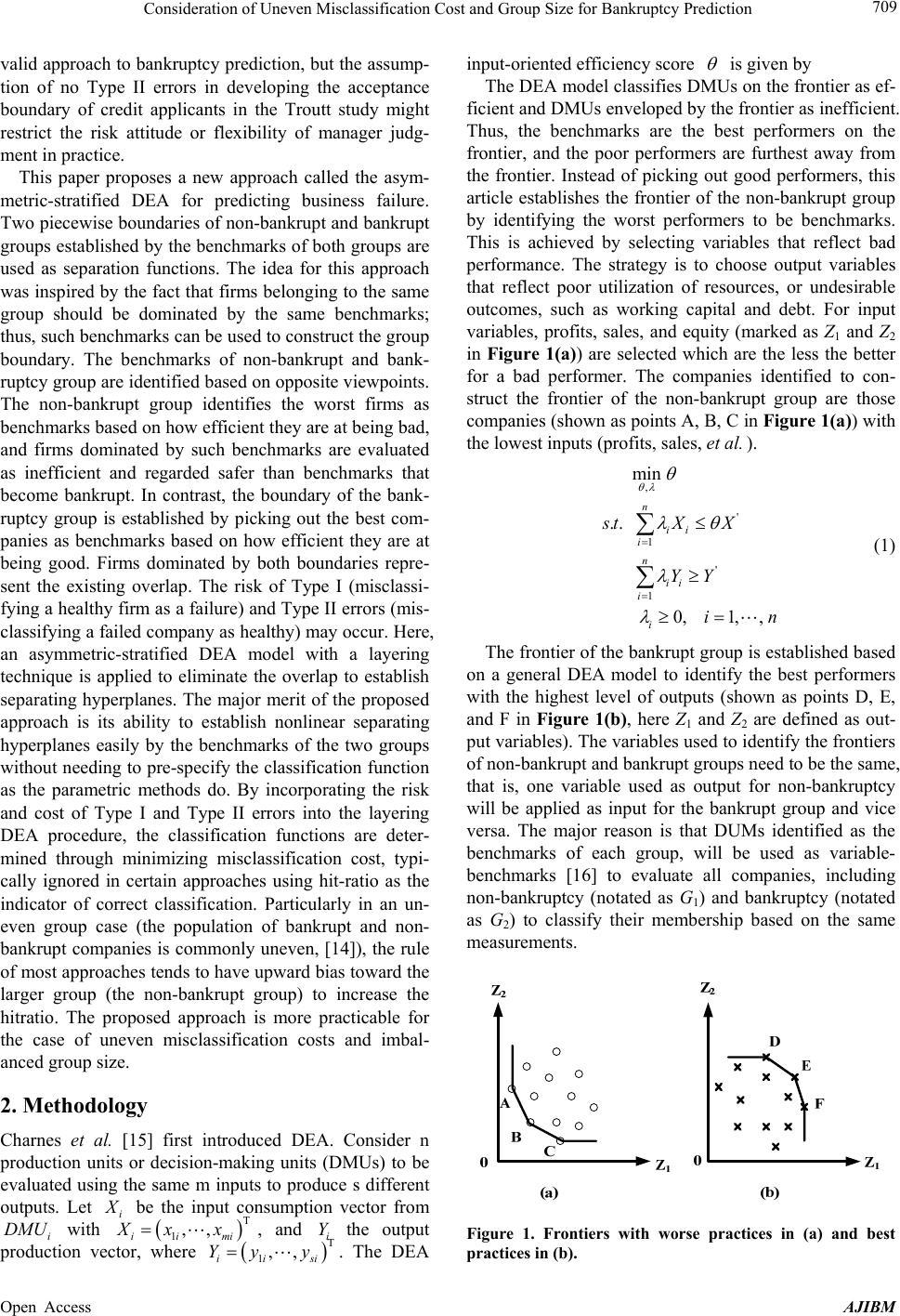

Consideration of Uneven Misclassification Cost and Group Size for Bankruptcy Prediction 709
valid approach to bankruptcy prediction, but the assump-
tion of no Type II errors in developing the acceptance
boundary of credit applicants in the Troutt study might
restrict the risk attitude or flexibility of manager judg-
ment in practice.
This paper proposes a new approach called the asym-
metric-stratified DEA for predicting business failure.
Two piecewise boundaries of non-bankrupt and bankrupt
groups established by the benchmarks of both groups are
used as separation functions. The idea for this approach
was inspired by the fact that firms belonging to the same
group should be dominated by the same benchmarks;
thus, such benchmarks can be used to construct the group
boundary. The benchmarks of non-bankrupt and bank-
ruptcy group are identified based on opposite viewpoints.
The non-bankrupt group identifies the worst firms as
benchmarks based on how efficient they are at being bad,
and firms dominated by such benchmarks are evaluated
as inefficient and regarded safer than benchmarks that
become bankrupt. In contrast, the boundary of the bank-
ruptcy group is established by picking out the best com-
panies as benchmarks based on how efficient they are at
being good. Firms dominated by both boundaries repre-
sent the existing overlap. The risk of Type I (misclassi-
fying a healthy firm as a failure) and Type II errors (mis-
classifying a failed company as healthy) may occur. Here,
an asymmetric-stratified DEA model with a layering
technique is applied to eliminate the overlap to establish
separating hyperplanes. The major merit of the proposed
approach is its ability to establish nonlinear separating
hyperplanes easily by the benchmarks of the two groups
without needing to pre-specify the classification function
as the parametric methods do. By incorporating the risk
and cost of Type I and Type II errors into the layering
DEA procedure, the classification functions are deter-
mined through minimizing misclassification cost, typi-
cally ignored in certain approaches using hit-ratio as the
indicator of correct classification. Particularly in an un-
even group case (the population of bankrupt and non-
bankrupt companies is commonly uneven, [14]), the rule
of most approaches tends to have upward bias toward the
larger group (the non-bankrupt group) to increase the
hitratio. The proposed approach is more practicable for
the case of uneven misclassification costs and imbal-
anced group size.
2. Methodology
Charnes et al. [15] first introduced DEA. Consider n
production units or decision-making units (DMUs) to be
evaluated using the same m inputs to produce s different
outputs. Let i
X
be the input consumption vector from
i with , and the output
production vector, where . The DEA
input-oriented efficiency score
DMU

T
1,,
iimi
Xx x
1
Yy


i
YT
si
y

,,
ii


is given by
The DEA model classifies DMUs on the frontier as ef-
ficient and DMUs enveloped by the frontier as inefficient.
Thus, the benchmarks are the best performers on the
frontier, and the poor performers are furthest away from
the frontier. Instead of picking out good performers, this
article establishes the frontier of the non-bankrupt group
by identifying the worst performers to be benchmarks.
This is achieved by selecting variables that reflect bad
performance. The strategy is to choose output variables
that reflect poor utilization of resources, or undesirable
outcomes, such as working capital and debt. For input
variables, profits, sales, and equity (marked as Z1 and Z2
in Figure 1(a)) are selected which are the less the better
for a bad performer. The companies identified to con-
struct the frontier of the non-bankrupt group are those
companies (shown as points A, B, C in Figure 1(a)) with
the lowest inputs (profits, sales, et al. ).
,
'
1
1
min
..
0,1,,
n
ii
i
n
ii
i
i
stX X
in










'
YY
 

(1)
The frontier of the bankrupt group is established based
on a general DEA model to identify the best performers
with the highest level of outputs (shown as points D, E,
and F in Figure 1(b), here Z1 and Z2 are defined as out-
put variables). The variables used to identify th e frontiers
of non-bankrupt and bankrupt groups need to be the same,
that is, one variable used as output for non-bankruptcy
will be applied as input for the bankrupt group and vice
versa. The major reason is that DUMs identified as the
benchmarks of each group, will be used as variable-
benchmarks [16] to evaluate all companies, including
non-bankruptcy (notated as G1) and bankruptcy (notated
as G2) to classify their membership based on the same
measurements.
Figure 1. Frontiers with worse practices in (a) and best
practices in (b).
Open Access AJIBM

Consideration of Uneven Misclassification Cost and Group Size for Bankruptcy Prediction
710
Define 1

1
,1,2,,
j
J
DMU jn for all the
DMUs of G1 (The same definition for G2). The set *
E
represents the benchmarks identified by model (1) where

*11
kk
EDMUJ  . If of one grou p is used as
the benchmark to evaluate all DMUs, is referred to as
the variable-benchmark. The variable benchmark model
for G1 is formulated below: (The formula is the same for
G2)
*
E*
E
1
1
*
*
new
new
*
min
..
0,
G
ipiG p
iE
iri r
iE
i
s
txx
yy
iE










 (2)
The efficiency score

is expressed as a number
between 0 - 1. A with a score less than one is
deemed inefficient relative to other DMUs. A company
evaluated to be inefficient by the variable-benchmarks of
one frontier, is dominated by such a frontier. Those
companies dominated by the same frontier are in the
same production possibility set (PPS) and classified to
the same group. Two PPSs of G1 and G2 might have an
intersection 2
new
DMU

1
1

1
P
PS PPS (shown as the shadow area
in Figure 2), which means some companies or DMUs
are dominated by the frontiers of G1 and G2 simultane-
ously, which may result in misclassification. That is, if
1
G

and 2
G

are the efficiency scores of
evaluated separately by the variable-benchmarks of G1
and G2, there will be four possible situations:
new
DMU




12
12
12
12
i.1, 1
ii .1,1
iii .1,1
iv .1,1
GG
GG
GG
GG








(3)
Situation (iii) indicates the intersection between two
PPSs because is dominated by the benchmarks
of G1 and G2simultaneously. To establish a general dis-
criminant rule that a company can be classified to a des-
new
DMU
Figure 2. Intersection (the shadow area) between the two
groups.
ignated group if it is dominated only by a correspondent
frontier, the stratification model [16] is further applied to
deal with the overlap problem.
Define


1
,1,2,,
lj
J
DMU jn
ll
for all the
DMUs of G1 (The same definition and process are for
G2). 1l
J
JE


, where



*,1 l
lk
l
k
EDMUJ 

 and is the
optimal value of the following model whenis un-
der evaluation.

*,lk

DMU

k








*
,,
,min,
.. ,
0,
i
l
l
lk
ipi pk
iFJ
iri rk
iFJ
l
i
lk lk
s
txl
yy
iFJ













kx
(4)
where


l
iFJ means . If
l
j
DMU J1l

, model
(4) is the original DEA model, and El consists of the
benchmarks. The DMUs in set El define the first layer of
the frontier. Two sets of El identified for two groups are
applied as variable-benchmarks to evaluate the efficiency
of all DMUs by model (3). If situation (iii) exists, model
(4) needs to be resolved by setting l = 2. By removing the
first layer of frontiers (marked G1(1) and G2(1) in Figure
3), some DMUs within the set of2
, are fur-
ther identified as benchmarks to form the second layer of
frontiers (marked G1(2) and G2(2)). The new PPSs (here
referred to as and), dominated by G1(2) and
G2(2), are the subset of and , making a
smaller intersection (notated as12
) between
them. The process needs to be performed from l = 1 to l
= L, where the layers of frontiers dominate two
subsets of PPSs having no intersection between them
1
1
P
PPS
2
P
1
PPS
2
2
PPS 1
1
PPS PPS 
PS
1
22
PS
2
1
th
PPS
L


12
LL
PPSPPS


. Then, these two layers of
frontiers can be applied as discriminant hyperplanes for
classification.
th
L
The stratification DEA model mentioned above is
performed based on a symmetric layering technique that
is suitable for an even size of both groups [17,18]. For
the bankruptcy prediction, removing a layer of the fron-
tier from the non-bankrupt group will raise the risk of
Type I error because of the reduced PPS range. If the
frontier being removed is from the bankrupt group , it will
increase the risk of Type II error. Generally, the cost of
Type II error is much more expensive than the Type I
error. To minimize the total cost of misclassification, an
asymmetric layering technique is performed by incorpo-
rating error costs and risk rates into the expected cost of
the misclassification (ECM) function to identify a pair of
frontiers that can minimize the misclassification cost.
That is:




12
min2 1211 21 2ECMcP pcP p (5)
Open Access AJIBM

Consideration of Uneven Misclassification Cost and Group Size for Bankruptcy Prediction 711
Figure 3. Two feasibilities of separating hyperplanes (G1(2) −
G2(2) and G1(3) − G2(1)).
where

21c

is the cost of Type I error and


12c
means the cost of Type II error.

21P and


12P
are the risk rates of Type I and Type II errors, calculated
with the accumulative number of benchmarks on the re-
moved frontiers, divided by the total amount of DMUs in
the corresponding group. The more frontiers removed
from the PPSs, the greater the risk of Type I or Type II
errors. The ratios of 1 and 2 are the proportions of
non-bankrupt and bankrupt companies. Several combina-
tions of the two sets of benchmarks (notated as
and ) can dominate two PPSs having no intersection
between them 12 . All have
various layers of removed frontiers on the two PPSs,
which cause different risks of
p

p

12
12
LL
*
1
E
*
2
E

,PPSPPSL L  

21P and


12P. An
optimal set of and is obtained by solving
model (5) to minimize the expected cost of misclassifica-
tion. Then, the frontiers constructed by and are
applied as discriminant hyperplanes, used to predict a
new observation by the variable-benchmark DEA model
(2). The rules of classification are:
*
1
E*
2
E
*
1
E*
2
E




12
12
12 12
12 12
** 1
** 2
** **new
1
** **new
2
Ifi1,1, then,
ii1,1,then,
iii1,1, and,then,
iv1,1,and,then.
new
GG
new
GG
GG GG
GG GG
DMU G
DMU G
DMU G
DMU G


 
 
 
 
 
 
(6)
3. Application
A data set containing annual financial data was collected
from Taiwan Stock Exchange for both failed and healthy
companies in 2006 and 2007. Nineteen and eleven failed
companies were matched with 160 and 115 healthy
companies in the two years to present an uneven group
size of the classification problem.
This study considered the 2006 data as training sam-
ples for model development and the 2007 data as holdout
samples for validation purposes. This article examined
the variables of total assets (TA), earnin gs before in come,
tax, depreciation and amortization (EBITDA), total cur-
rent liabilities (CL), interest expense (IN), and cash flow
from operations (CF) to be different significantly be-
tween bankrupt and non-bankrupt groups and selected
them as discriminant factors.
To identify the worst performers to establish the
boundary for the non-bankrupt group, those DUMs with
the highest output of total assets (TA), total current li-
abilities (CL), and interest expense (IN) while having the
lowest input level of earnings before income, tax, depre-
ciation and amortization (EBITDA) and cash flow (CF),
were identified as benchmarks. The same variables were
used by define TA, CL and IN as input variables, and
EBITDA and CF as output for the bankrupt group to
identify the best performers. Because negative value is
typical for some financial variables, to satisfy the posi-
tive restriction in the DEA model, any one of the selected
factors taking on a negative value needs to add an ade-
quate positive constant value to the factor value of all
DMUs with the absolute value of the most negative value
among those DMUs plus one. Two sets of benchmarks
identified by the DEA model (1) with the aforementioned
variables were applied to evaluate all DMUs by the vari-
able-benchmark DEA model (2). The results indicated
the existence of an overlap, because there were 64 DMUs
dominated simultaneously by the first layers of the two
groups, eight DMUs from bankruptcy, and 56 from
non-bankruptcy. To eliminate the intersection, sequential
layers of frontier were generated for non-bankrupt and
bankrupt groups by performing the stratification DEA
model (3). Tables 1 and 2 show the number of identified
benchmarks in each layer of frontier and the risk occur-
ring from the removed frontiers.
Because the sample of non-bankrupt and bankrupt
companies is uneven, the number of layers of the re-
moved frontiers is unequal. Tables 1 and 2 show that
removing nine layers of frontier can move 100% of failed
companies out of the PPS, while only 30% of the healthy
companies were removed from the non-bankruptcy group.
It is significant that the risks caused by the removed
frontiers differ between the two groups. Removing a
layer of frontier from the bankrupt group creates much
more risk (Type II errors) than from the non-bankruptcy
group (Type I errors), because the first layer of removed
frontier caus es only 1.25% r isk in non- b ankruptcy (Type
I errors) but 10.53% in bankruptcy (Type II errors). Eight
collocations of pair frontiers can make no intersection
between two PPSs of non-bankrupt and bankrupt groups.
To identify the optimal pair of frontiers to be separating
hyperplanes, formula (5) is solved in accordance with
different error risks and costs caused from each colloca-
tion to minimize expected cost of misclassification.
There are eight collocations of pair frontiers making
no intersection between two PPSs of non-bankrupt and
bankrupt group s. To identify the optimal pair of frontiers
to be separating hyperplanes, formula (5) is solved in
Open Access AJIBM

Consideration of Uneven Misclassification Cost and Group Size for Bankruptcy Prediction
Open Access AJIBM
712
Table 1. The number of identified benchmarks on each frontier and the risk occurred from the removed frontiers of non-
bankrupt group.
Layer Number of
Benchmarks
Accumulative
Number of Removed
Benchmarks
Accumulative
Risk of Error


21P % Layer Number of
Benchmarks
Accumulative
Number of Removed
Benchmarks
Accumulative
Risk of Error


21P %
1 2 0 0.00 12 7 63 39.38
2 3 2 1.25 13 8 70 43.75
3 4 5 3.13 14 11 78 48.75
4 9 9 5.63 15 7 89 55.63
5 5 18 11.25 16 6 96 60.00
6 4 23 14.38 17 8 102 63.75
7 6 27 16.88 18 6 110 68.75
8 8 33 20.63 19 9 116 72.50
9 7 41 30.00 20 5 125 78.13
10 10 48 36.25 21 4 130 81.25
11 5 58 39.38 134 83.75
Table 2. The number of identified benchmarks on each frontier and the risk occurred from the removed frontiers of bank-
rupt group.
Layer Number of
Benchmarks
Accumulative
Number of Removed
Benchmarks
Accumulative
Risk of Error


12P % Layer Number of
Benchmarks
Accumulative
Number of Removed
Benchmarks
Accumulative
Risk of Error


12P %
1 2 0 0.00 6 1 13 68.42
2 2 2 10.53 7 1 14 73.68
3 3 4 21.05 8 2 15 78.95
4 3 7 36.84 9 2 17 89.47
5 3 10 52.63 19 100.00
accordance with different error risks and costs caused
from each collocation to minimize expected cost of mis-
classification. The ratio of Type II cost to Type I cost
 
12 21cc

is assumed from 1 to 1 to 20 to 1 for
the situation of different applications. Table 3 shows
NB-2 and B-7 are the best choice if ignoring the influ-
ence of error cost (that is, assume

12 21cc
equal
to 1). For which, only 1.25% of healthy companies (the
benchmarks on the first layer of frontier, see Table 1) are
removed from the non-bankrupt group, but 78.95% of
failed companies (the benchmarks removed from layer
one to layer six, see Table 2) need to be removed from
the bankrupt group because the classification accuracy of
the smaller group is sacrificed to increase the hit-ratio. If
Type II cost is much higher than Type I cost (as Table 3
shows, 20 times to Type I cost), the pair frontiers of
NB-21 and B-1 is the best selection for the purpose of
minimizing expected misclassification cost. Besides, if
the pair of frontiers is determined by the symmetric-
stratified DEA model, that is, remove the same number
of layers from both groups, the misclassification cost is
almost higher than the lowest value of all collocations
determined by the asymmetric-stratified model. In ac-
cordance with the empirical studies of Altman (1993)
and Hull (1998), the cost of Type II errors is in the rang e
of 0.6 to 0.7 and Type I errors are derived from the in-
terest spread of usually 3% - 5%. Therefore, this article
assumed that Type II cost is 20 times to Type I cost, and
the pair frontiers of NB-21 and B-1 were then the best
selection to be discrimination hyperplanes for further
analysis and discussion.
Table 4 shows the hit-ratios of training and holdout
data. If the purpose is to maximize the hit-ratio, the fron-
tiers of NB-2 and B-7 are the best choice with the
hit-ratios of 94.44% on training and 91.67% on hold out
samples. High prediction accuracy supports the validity
of the proposed DEA approach, a result consistent with
some traditional discriminant methods whose analyses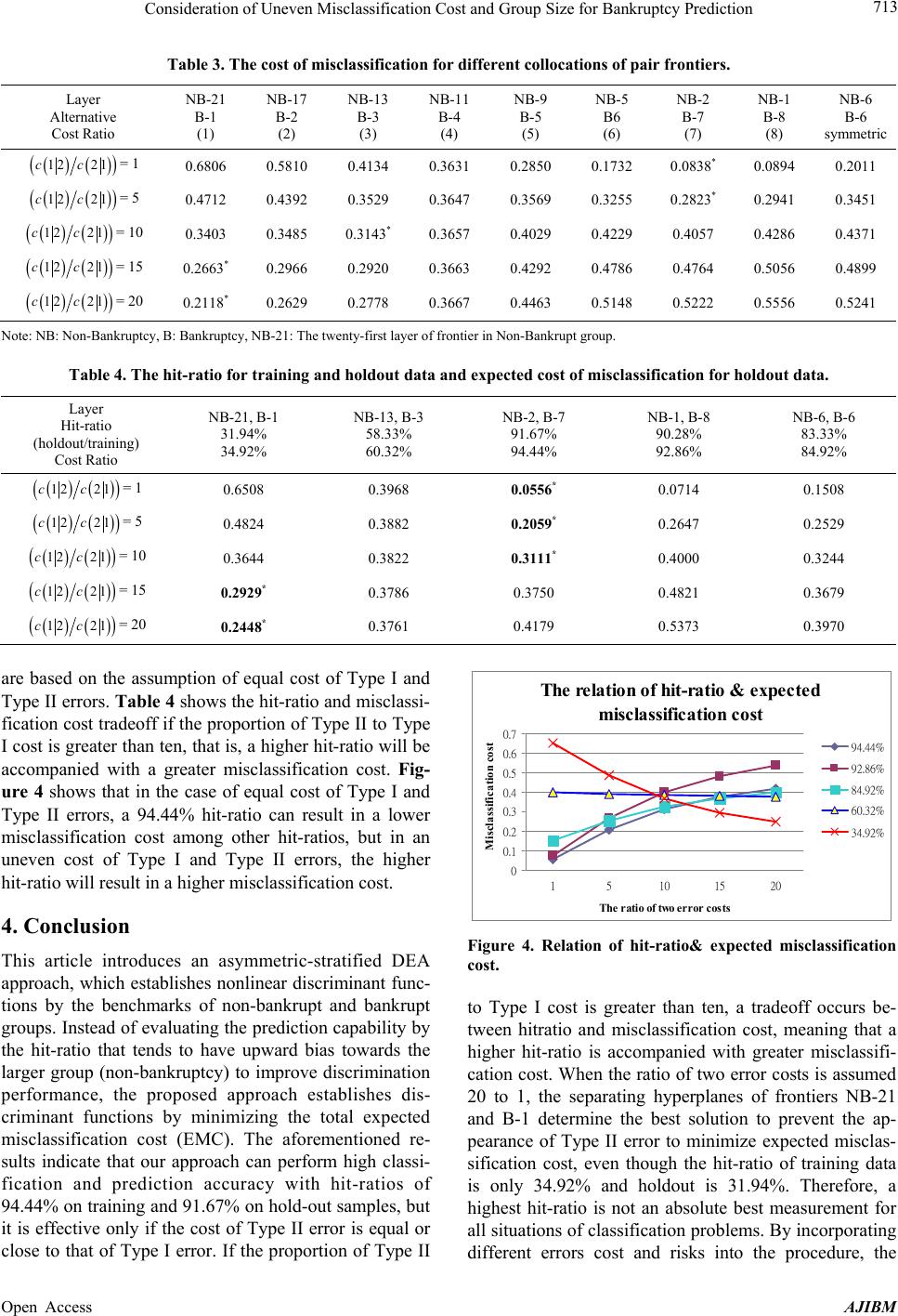

Consideration of Uneven Misclassification Cost and Group Size for Bankruptcy Prediction 713
Table 3. The cost of misclassification for different collocations of pair frontiers.
Layer
Alternative
Cost Ratio
NB-21
B-1
(1)
NB-17
B-2
(2)
NB-13
B-3
(3)
NB-11
B-4
(4)
NB-9
B-5
(5)
NB-5
B6
(6)
NB-2
B-7
(7)
NB-1
B-8
(8)
NB-6
B-6
symmetric






12 21cc= 1 0.6806 0.5810 0.4134 0.3631 0.2850 0.1732 0.0838* 0.0894 0.2011






12 21cc= 5 0.4712 0.4392 0.3529 0.3647 0.3569 0.3255 0.2823* 0.2941 0.3451






12 21cc= 10 0.3403 0.3485 0.3143* 0.3657 0.4029 0.4229 0.4057 0.4286 0.4371






12 21cc= 15 0.2663* 0.2966 0.2920 0.3663 0.4292 0.4786 0.4764 0.5056 0.4899






12 21cc= 20 0.2118* 0.2629 0.2778 0.3667 0.4463 0.5148 0.5222 0.5556 0.5241
Note: NB: Non-Bankruptcy, B: Bankruptcy, NB-21 : The twenty-first layer of frontier in Non-Bankrupt group.
Table 4. The hit-ratio for training and holdout data and expected cost of misclassification for holdout data.
Layer
Hit-ratio
(holdout/training)
Cost Ratio
NB-21, B-1
31.94%
34.92%
NB-13, B-3
58.33%
60.32%
NB-2, B-7
91.67%
94.44%
NB-1, B-8
90.28%
92.86%
NB-6, B-6
83.33%
84.92%






12 21cc= 1 0.6508 0.3968 0.0556* 0.0714 0.1508






12 21cc= 5 0.4824 0.3882 0.2059* 0.2647 0.2529






12 21cc= 10 0.3644 0.3822 0.3111* 0.4000 0.3244






12 21cc= 15 0.2929* 0.3786 0.3750 0.4821 0.3679






12 21cc= 20 0.2448* 0.3761 0.4179 0.5373 0.3970
are based on the assumption of equal cost of Type I and
Type II errors. Table 4 shows the hit-ratio and misclassi-
fication cost tradeoff if the proportion of Type II to Type
I cost is greater than ten, that is, a higher hit-ratio will be
accompanied with a greater misclassification cost. Fig-
ure 4 shows that in the case of equal cost of Type I and
Type II errors, a 94.44% hit-ratio can result in a lower
misclassification cost among other hit-ratios, but in an
uneven cost of Type I and Type II errors, the higher
hit-ratio will result in a higher misclassification cost.
4. Conclusion
This article introduces an asymmetric-stratified DEA
approach, which establishes nonlinear discriminant func-
tions by the benchmarks of non-bankrupt and bankrupt
groups. Instead of evaluating the prediction capability by
the hit-ratio that tends to have upward bias towards the
larger group (non-bankruptcy) to improve discrimination
performance, the proposed approach establishes dis-
criminant functions by minimizing the total expected
misclassification cost (EMC). The aforementioned re-
sults indicate that our approach can perform high classi-
fication and prediction accuracy with hit-ratios of
94.44% on training an d 91.67% on hold-out samples, but
it is effective only if the cost of Type II error is equal or
close to that of Type I error. If the proportion of Type II
The relation of hit-ratio & expected
misclassification cost
0
0.1
0.2
0.3
0.4
0.5
0.6
0.7
1510 15 20
The ratio of two error costs
Misclassification cost
94.44%
92.86%
84.92%
60.32%
34.92%
Figure 4. Relation of hit-ratio& expected misclassification
cost.
to Type I cost is greater than ten, a tradeoff occurs be-
tween hitratio and misclassification cost, meaning that a
higher hit-ratio is accompanied with greater misclassifi-
cation cost. When the ratio of two error costs is assumed
20 to 1, the separating hyperplanes of frontiers NB-21
and B-1 determine the best solution to prevent the ap-
pearance of Type II error to minimize expected misclas-
sification cost, even though the hit-ratio of training data
is only 34.92% and holdout is 31.94%. Therefore, a
highest hit-ratio is not an absolute best measurement for
all situations of classification problems. By incorporating
different errors cost and risks into the procedure, the
Open Access AJIBM

Consideration of Uneven Misclassification Cost and Group Size for Bankruptcy Prediction
714
proposed benchmark approach can easily establish more
than one separating hyperplane and provide flexibility to
decision makers for credit evaluation and bankruptcy
prediction.
REFERENCES
[1] E. I. Altman, “Financial Ratios, Discriminant Analysis
and the Prediction of Corporate Bankruptcy,” The Journal
of Finance, Vol. 23, No. 4, 1968, pp. 589-609.
http://dx.doi.org/10.1111/j.1540-6261.1968.tb00843.x
[2] A. I. Dimitras, C. Zopounidis and C. Hurson, “A Multic-
riteria Decision Aid Method for the Assessment of Busi-
ness Failure Risk,” Foundations of Computing and Deci-
sion Sciences, Vol. 20, No. 2, 1995, pp. 99-112.
[3] A. I. Dimitras, S. H. Zanakis and C. Zopounidis, “A Sur-
vey of Business Failures with an Emphasis on Prediction
Methods and Industrial Applications,” European Journal
of Operation Research, Vol. 90, No. 3, 1996, pp. 487-513.
http://dx.doi.org/10.1016/0377-2217(95)00070-4
[4] B. E. Deakin, “A Discriminant Analysis of Predictors of
Business Failure,” Journal of Accounting Re search Spring,
Vol. 10, No. 1, 1976, pp.167-179.
[5] M. D. Troutt, A. Rai and A. Zhang, “The Potential Use of
DEA for Credit Applicant Acceptance Systems,” Com-
puters Operations Research, Vol. 23, No. 4, 1996, pp.
405-408.
http://dx.doi.org/10.1016/0305-0548(95)00048-8
[6] D. Retzlaff-Roberts and R. Puelz, “Classification in Auto-
mobile Insurance Using a DEA and Discriminant Analy-
sis Hybrid,” Journal of Productivity Analysis, Vol. 7, No.
4, 1996, pp. 417-427.
http://dx.doi.org/10.1007/BF00162050
[7] L. M. Seiford and J. Zhu, “An Acceptance System Deci-
sion Rule with Data Envelopment Analysis,” Computers
Operations Research, Vol. 25, No. 4, 1998, pp. 329-332.
http://dx.doi.org/10.1016/S0305-0548(97)00075-0
[8] P. C. Pendharkar, “A Potential Use of Data Envelopment
Analysis for the Inverse Classification Problem,” Omega,
Vol. 30, No. 3, 2002, pp. 243-248.
http://dx.doi.org/10.1016/S0305-0483(02)00030-0
[9] A. Cielen, L. Peeters and K. Vanhoof, “Bankruptcy Pre-
diction Using a Data Envelopment Analysis,” European
Journal of Operational Research, Vol. 154, No. 2, 2004,
pp. 526-532.
http://dx.doi.org/10.1016/S0377-2217(03)00186-3
[10] J. C. Paradi, M. Asmild and P. C. Simak, “Using DEA
and Worst Practice DEA in Credit Risk Evaluation,” Jour-
nal of Productivity Analysis, Vol. 21, No. 2, 2004, pp.
153-165.
http://dx.doi.org/10.1023/B:PROD.0000016870.47060.0b
[11] T. Sueyoshi and M. Goto, “DEA-Discriminant Analysis:
Methodological Comparison Among Eight Discriminant
Analysis Approaches,” European Journal of Operational
Research, Vol. 169, No. 1, 2006, pp. 247-272.
http://dx.doi.org/10.1016/j.ejor.2004.05.025
[12] T. Sueyoshi and M. Goto, “DEA-DA for Bankruptcy-
Based Performance Assessme nt: Misclassification Analy-
sis of Japanese Construction Industry ,” European Journal
of Operational Research, Vol. 199, No. 2, 2009, pp. 576-
594. http://dx.doi.org/10.1016/j.ejor.2008.11.039
[13] M. Psillaki, I. E. Tsolas and D. Margaritis, “Evaluation of
Credit Risk Based on Firm Performance,” European
Journal of Operational Research, Vol. 201, No. 3, 2010,
pp. 873-881. http://dx.doi.org/10.1016/j.ejor.2009.03.032
[14] A. Charnes and W. W. Cooper, “Goal Programming and
Multiple Objective Optimization,” European Journal of
Operational Research, Vol. 1, No. 1, 1977, pp. 39-54.
http://dx.doi.org/10.1016/S0377-2217(77)81007-2
[15] A. Charnes, W. W. Cooper and E. Rhode, “Measuring the
Efficiency of Decision Making Units,” European Journal
of Operational Research, Vol. 2, No. 6, 1978, pp. 429-
444. http://dx.doi.org/10.1016/0377-2217(78)90138-8
[16] J. Zhu, “Quantitative Models for Performance Evaluation
and Benchmarking: Data Envelopment Analysis with
Spreadsheets and DEA Excel Solver,” Kluwer Academic
Publishers, Boston, 2003.
http://dx.doi.org/10.1007/978-1-4757-4246-6
[17] D. S. Chang and Y. I. Kuo, “A Novel Procedure to Iden-
tify the Minimized Overlap Boundary of Two Groups by
DEA Model,” Lecture Notes in Computer Science, Vol.
3483, 2005, pp. 577-586.
http://dx.doi.org/10.1007/11424925_61
[18] D. S. Chang and Y. I. Kuo, “An Approach for the Two-
Group Discriminant Analysis: An Application of DEA,”
Mathematic & Computer Modelling, Vol. 47, No. 9-10,
2008, pp. 970-981.
http://dx.doi.org/10.1016/j.mcm.2007.05.010
Open Access AJIBM