Application of Propagation Modeling to Verify and Discriminate Ground-Truth Infrasound Signals at Regional Distances

doi:10.4236/inframatics.2013.24004

Paper Menu >>

Journal Menu >>

InfraMatics, 2013, 2, 39-55

Published Online December 2013 (http://www.scirp.org/journal/inframatics)

http://dx.doi.org/10.4236/inframatics.2013.24004

Open Access InfraMatics

Application of Propagation Modeling to Verify and

Discriminate Ground-Truth Infrasound Signals

at Regional Distances

Christoph Pilger1, Florian Streicher2, Lars Ceranna1, Karl Koch1

1Federal Institute for Geosciences and Natural Resources (BGR), Hannover, Germany

2German Aerospace Center (DLR), Oberpfaffenhofen, Germany

Email: christoph.pilger@bgr.de

Received November 5, 2013; revised December 11, 2013; accepted December 18, 2013

which permits unrestricted use, distribution, and reproduction in any medium, provided the original work is properly cited. In accor-

ABSTRACT

An infrasound field campaign was performed in 2011/2012 utilizing single infrasound sensors along the great circle

path between a known ground-truth source (Ariane 5 engine test facility, Lampoldshausen, Germany) and a regional

receiver (German infrasound array IS26, Bavarian Forest) covering a distance of rough 320 km in total. The gathered

recordings provide new insights in the infrasonic wave propagation at regional and near-source distances by comparing

measured signals with modeling results within this study. Ray-tracing and parabolic equation approaches are utilized to

model infrasound propagation from the ground-truth source to the line profile sensors and explain the obtained detec-

tions and non-detections. Modeling and observation results are compared by estimating their amplitude, quantifying

amplitude deviations and also considering observed and calculated travel times and celerities. Modeling results show a

significant influence of small-scale atmospheric variations in effective sound speed profiles on the propagation pattern,

which results in varying tropospheric and stratospheric ducting behavior. A large number of gravity wave profiles are

tested to investigate the influences of atmospheric dynamics on the infrasound wave field and improve the modeling

results. The modeling is furthermore applied to a case of two potential, contemporaneous and closely spaced infrasound

sources. Propagation modeling is used here to resolve the source ambiguity between a ground-based and a higher alti-

tude source giving a strong preference to the latter with respect to the observed infrasonic signatures. The good agree-

ment between modeling and observation results within this study successfully shows the benefit of applying infrasound

propagation modeling to the validation of infrasound measurements, verification of ducting behavior and discrimination

of infrasound sources.

Keywords: Infrasound; Propagation Modeling; Ground-Truth

1. Introduction

Infrasound is generated by a variety of different natural

and artificial sources such as volcanic eruptions or mete-

orite entries [1-3] and anthropogenic events such as air-

craft/spacecraft signatures or explosions [4-6], respec-

tively. Infrasonic signals from different sources are de-

tected by microbarometers at nearby up to very remote

distances (e.g. see [7-9]). Usually, when an infrasonic

detection is made, the corresponding source is unknown

and can be identified by quantifying arrival time, signal

frequency, amplitude, velocity and back-azimuth [10].

However, difficulties in the proper source identification

are due to uncertainties introduced by atmospheric varia-

tions on the source-to-receiver propagation path, signal-

to-noise issues and ambiguities in active infrasound

sources in the source direction.

In contrast, ground-truth sources are events with well-

known source parameters such as time and exact location,

or clearly observed by complementary techniques, so

they have well-known back-azimuths and distances from

source to receiver. In this case, travel-time and celerity

for an observed signal can be quantified and thus addi-

tional information is available on how the signal was

ducted from the source to a receiver. Alternatively, in-

C. PILGER ET AL.

formation about the atmospheric conditions on the prop-

agation path can be acquired or verified by inverting ob-

served waveforms and their parameters from ground-

truth sources (e.g., [11-13]).

Infrasound propagation modeling (e.g., [14,15]) is

used to describe the propagation pattern of infrasonic

signatures from a surface or elevated source to a receiv-

ing instrument. Aspects of ducting through different alti-

tudes of the atmosphere (troposphere, stratosphere or ther-

mosphere), the extent of shadow zones as well as estima-

tion of amplitudes and sound attenuation can be covered

[16-18]. Propagation modeling is applied in this study to

verify ducting from a known ground-truth source to a

receiver and to discriminate between different potential

sources of a signature, also taking into consideration at-

mospheric conditions and small-scale changes on the

propagation path. Certain detections and their observed

travel-time and celerity values can only be explained by

including unusual propagation conditions, near-field tro-

pospheric ducting and small-scale atmospheric perturba-

tions such as gravity waves [19-22].

In Section 2 of this study, the observational setting of

Ariane 5 rocket engine tests as a ground-truth source [23]

and infrasound measurements on a line profile of micro-

barometers towards an infrasound array as measurement

setting are described. Two different propagation models,

a ray-tracing [24] and a parabolic equation approach [25],

described in Section 3, are applied to study infrasonic

source-to-receiver paths. Atmospheric background mod-

els using ECMWF analysis data, climatologies and fine-

scale gravity wave structures are included for a realistic

estimation of wave ducting. In Section 4, results are de-

scribed and discussed concerning tropospheric and stra-

tospheric wave ducting, estimation of source amplitudes

and consideration of atmospheric dynamics. Finally, in

Section 5, all results are summarized and conclusions are

given.

2. Measurements

In a previous study [23], infrasound signals were analyz-

ed from Ariane 5 engine tests in the years 2000-2004 that

could be identified at station IS26 of the International

Monitoring System (IMS) network of the Comprehensive

Nuclear-Test-Ban Treaty Organization (CTBTO). In

spring 2011, information was obtained that a new series

of engine tests was planned between fall 2011 and spring

2012 at the rocket propulsion testing facility of the Ger-

man Aerospace Center (DLR) near Heilbronn, Southern

Germany (49.287˚N, 9.378˚E). Since this setting was

favorable for recording these tests along the path to IS26

based on the prevailing winter wind conditions, as had

been found earlier [23,26], a field campaign was de-

signed to cover local propagation distances as close as 20

km to regional distances of IS26, at a range of 320 km.

The geographical setting for this field experiment is

shown in Figure 1 and a summary of the ground truth

information for the different tests is provided in Table 1.

Figure 1. Layout of the field campaign in two different setups (stations DLR1a to DLR6a, yellow triangles, from 20 to 120 km

and stations DLR1b to DLR6b, orange triangles, from 120 to 240 km). Also shown is the Ariane 5 engine test source (black

star) near Heilbronn, nearby seismometer and sound pressure level microphone (green triangle, DLR-P4), complementary

sources near Bitburg, Germany and in Luxemburg (black stars, BIT, LUX), seismometer stations near the sources (blue tri-

angles, SIND, RUP, ABH) and the IS26 infrasound array (red hexagon) near Passau.

Open Access InfraMatics

C. PILGER ET AL. 41

Table 1. Details of ground-truth information (in black) and observations (in green/red) for nine Ariane 5 rocket engine tests

and two additional potential sources (BIT, LUX, see text and Figure 1). Durations for the additional sources are not applica-

ble, since signals are assumed to be impulsive. Positive detections of the source by instruments at a given distance are shown

in green, non-detections in red. Instruments set-up but not in operation (and thus not capable of signal detections) are not

listed.

Test Nr. Date Start Time DurationSeismo-AcousticLine Profile Microbarometers IS26 station

1 18-11-2011 15:50 UTC 600 s 20 km - 320 km

2 08-12-2011 15:30 UTC 668 s 20 km - 320 km

3 19-12-2011 15:17 UTC 646 s 20 km 40 km, 60 km, 80 km, 100 km,120 km 320 km

4 16-01-2012 16:43 UTC 285 s 20 km 20 km, 40 km, 60 km, 80 km, 120 km 320 km

5 16-02-2012 13:28 UTC 720 s 20 km 20 km, 40 km, 60 km, 80 km, 120 km 320 km

6 07-03-2012 15:53 UTC 700 s 20 km 120 km, 160 km, 180 km, 210 km, 240 km 320 km

7 22-03-2012 15:31 UTC 696 s 20 km 120 km, 160 km, 180 km, 210 km, 240 km 320 km

8 27-04-2012 14:39 UTC 653 s 20 km 120 km, 140 km, 180 km 320 km

9 14-05-2012 15:21 UTC 530 s 20 km 120 km, 140 km, 160 km, 180 km 320 km

BIT 16-02-2012 11:19 UTC N/A 50 km, 60 km 240 km, 260 km, 280 km, 300 km, 340 km 530 km

LUX 16-02-2012 11:17 UTC N/A 70 km, 100 km 270 km, 290 km, 310 km, 330 km, 370 km 560 km

As only a limited number of six mobile infrasound re-

cording systems was available, a deployment plan was

devised to set up a linear station profile with inter-station

spacing of about 20 km in two distinct stages: for ap-

proximately half of the initially announced seven engine

tests in the distance range from 20 to 120 km and for the

remaining tests to cover, as much as possible, the gap of

ranges to IS26. In addition to the mobile infrasound sta-

tions we were able to obtain seismo-acoustic waveforms

from a seismometer station (SIND) operated by the State

Seismological Survey of Baden-Württemberg, Germany

(pers.comm.) which was located at a similar range as the

closest infrasound station at 20 km, and only at a slightly

different azimuth to the source. The specific distances

covered in every test can be found in Table 1. The given

listing shows that for the first two tests only recordings

from the seismometer station (SIND) and IS26 could be

obtained, as it was not possible to respond to short-term

announcements of these tests with field deployments.

However, since DLR announced two additional tests by

the time the original tests were concluded, the shorter

and the longer range station profiles were covered by

three and four engine tests, respectively.

The mobile infrasound equipment consisted of Reftek

digitizers and single MB-2000/2005 microbarometers per

site. For reducing wind noise for our installations in

harsh fall and winter conditions we connected porous

hoses of 5 - 8 m length to the microbarometers. Addi-

tional details on the deployed equipment and the wind

noise reduction filters used at the mobile stations are

given in [27]. Furthermore, we also put a seismometer

about 50 m from the engine testing facility to monitor the

ground-truth source and its temporal stability. For the

final test, the sound pressure level was also recorded by

the German Aerospace Center, Heilbronn (pers.comm.)

at about 24 m distance to the source. Concerning the

infrasound observations from the various tests (see Tabl e

1) and the different profile configurations we found in-

termittent instances for rather short distances (20 or 40

km), lack of signals for more than 40 km and less than

120 km, and fairly consistent signals at or beyond 120

km (except in one case) as well as at IS26 where all nine

tests were identified, as expected from a testing cam-

paign within winter months [23]. Only the April and May

2012 tests are somewhat extraordinary, because there had

not been any observations at IS26 such late in spring for

past engine tests. For the quantitative modeling attempt-

ed in this study the data were analyzed to determine tra-

vel times and pressure amplitudes. Spectral analysis of

line profile and IS26 data showed a dominant frequency

of 4 Hz, on which we based the modeling described be-

low. For the IS26 infrasound array we also carried out

frequency-wavenumber (FK) analyses to confirm the

proper azimuth of the signals.

During the field campaign an incidental observation of

yet another example of possible ground-truth sources

occurred. On 16 February 2012, a few hours prior to one

of the Ariane engine tests, rather significant infrasound

signals were recorded along the profile of sensors. In the

following days, there were media reports about an explo-

sion event in the Grand-Duchy of Luxemburg. The re-

ported site of this explosion was some 240 km further to

the west-northwest of the rocket testing facility and al-

most on the same great circle path of the recording pro-

Open Access InfraMatics

C. PILGER ET AL.

file towards IS26. At the same time there were also re-

ports about a potential sonic boom from a fighter aircraft

in the Western parts of Germany, in the Eifel region. The

German Air Force confirmed a supersonic flight in this

region and eventually provided corresponding ground-

truth information about the flight times and path of the

relevant aircraft (pers.comm.). The Luxemburg explosion

site and an estimated source location on the supersonic

aircraft’s flight path are also marked in Figure 1 (LUX,

BIT). The event was registered by two nearby seis-

mometer stations (ABH, RUP) of the State Seismological

Survey of Baden-Württemberg, Germany (pers.comm.),

on which the source location estimate of the aircraft was

based, along the line profile stations and at IS26 in a dis-

tance of more than 550 km. The corresponding distances

of the stations to these sources are given in Table 1. The

clear observations obtained from the source, either in

Luxemburg or over the Eifel region, certainly confirmed

the proper operation of the line profile stations that were

mostly deployed in the acoustic shadow zone for the

early propulsion tests.

3. Modeling

Infrasound propagation modeling is carried out within

this study to verify detections and non-detections ob-

tained along the line profile infrasound measurements

towards the IS26 array. It is also performed to identify

and discriminate complementary detections observed

during the field campaign.

Propagation modeling approaches utilized within this

study are the parabolic equation (PE) algorithm of the

software package InfraMAP [25] and the ray-tracing (RT)

method HARPA/DLR [24], an enhanced version of the

original HARPA ray-tracing program [28]. Realistic at-

mospheric background conditions are included in the

modeling by the use of ECMWF model analysis data

(www.ecmwf.int) combined with climatologies for hori-

zontal wind and temperatures above 60 km (HWM07, see

[29]; MSISE00, see [30]). Fine-scale atmospheric struc-

tures are introduced in the modeling by using gravity-

wave disturbances of the effective sound speed following

[31].

Figure 2 shows two-dimensional representations of

the PE and the RT methods for atmospheric infrasound

propagation paths between source and receiver(s). The

two methods are shown and described separately in this

section/figure, but in the course of the study both are

combined in a joint representation for most cases. This

should mainly highlight commonalities of the two meth-

ods in explaining observations and atmospheric states.

Nevertheless, slight differences evident in the compari-

son of both methods are due to their different approaches

(parabolic vs. Hamilton equations), different dimension-

alities of modeling space (two-dimensional PE vs. three

dimensional RT, of which only two-dimensional projec-

tions are shown within this study) and background rep-

resentations (one-dimensional temperature and wind pro-

file for PE vs. four-dimensional temperature and wind

fields for RT). One particular difference is the presence

of a weak PE infrasound field that scatters outside the RT

ray tubes into shadow zones (e.g. the range between 30

km and 120 km in Figure 2). No ray paths are predicted

in this region, but a PE amplitude of about −60 dB is

modeled. This is due to small amounts of wave energy

leaking from wave ducts and scattering into the shadow-

zone (e.g., [19,21]); a process which can be represented

by the used PE but not RT methods. Another difference

is a slight horizontal shift of rays returning from the stra-

tosphere in some of the test cases. These differences are

inevitable due to the available model versions, but also

allow consideration and discussion of infrasound propa-

gation and atmospheric effects on different scales (see

Section 4). The main outputs by the two methods are

range-height-fields of infrasound wave amplitude for PE

and range-height-views of ray patterns for RT, both

modeled for a frequency of 4 Hz identified as the domi-

nant signal frequency (see Section 2). Further model

outputs of surface pressure amplitudes, travel times and

celerities are introduced in Section 4.

Atmospheric background parameters, which are essen-

tial for the propagation of infrasound, are temperature,

zonal and meridional winds from the ground to thermos-

pheric altitudes above 120 km. The effective sound speed,

which combines temperature (by temperature-dependent

sound-speed) and wind (in the direction of infrasound

propagation) into one parameter, controls ducting of in-

frasound between surface and certain altitudes as e.g. the

troposphere, stratosphere and thermosphere. Additional

fine-scale structure, e.g. by atmospheric dynamics like

gravity waves (see [32]), can furthermore change the

effective sound speed and thus modify ducting behavior.

Figure 3 shows an exemplary profile of temperature and

winds derived from ECMWF, HWM and MSISE as well

as the resulting effective sound speed with and without

an arbitrary gravity-wave perturbation.

4. Results and Discussion

The propagation of infrasound can be subdivided in tro-

pospheric, stratospheric and thermospheric ducts as well

as rays escaping the atmosphere [14]. Due to the high

signal frequencies of the observations in this study (about

4 Hz) and correspondingly increased attenuation in the

upper atmosphere, no thermospheric returns are expected

or observed.

Detections of Ariane 5 rocket engine signals in the

infrasound frequency range have been found during the

field campaign at distances from 20 to 320 km. Tropo-

spheric arrivals have been observed in the near field be-

Open Access InfraMatics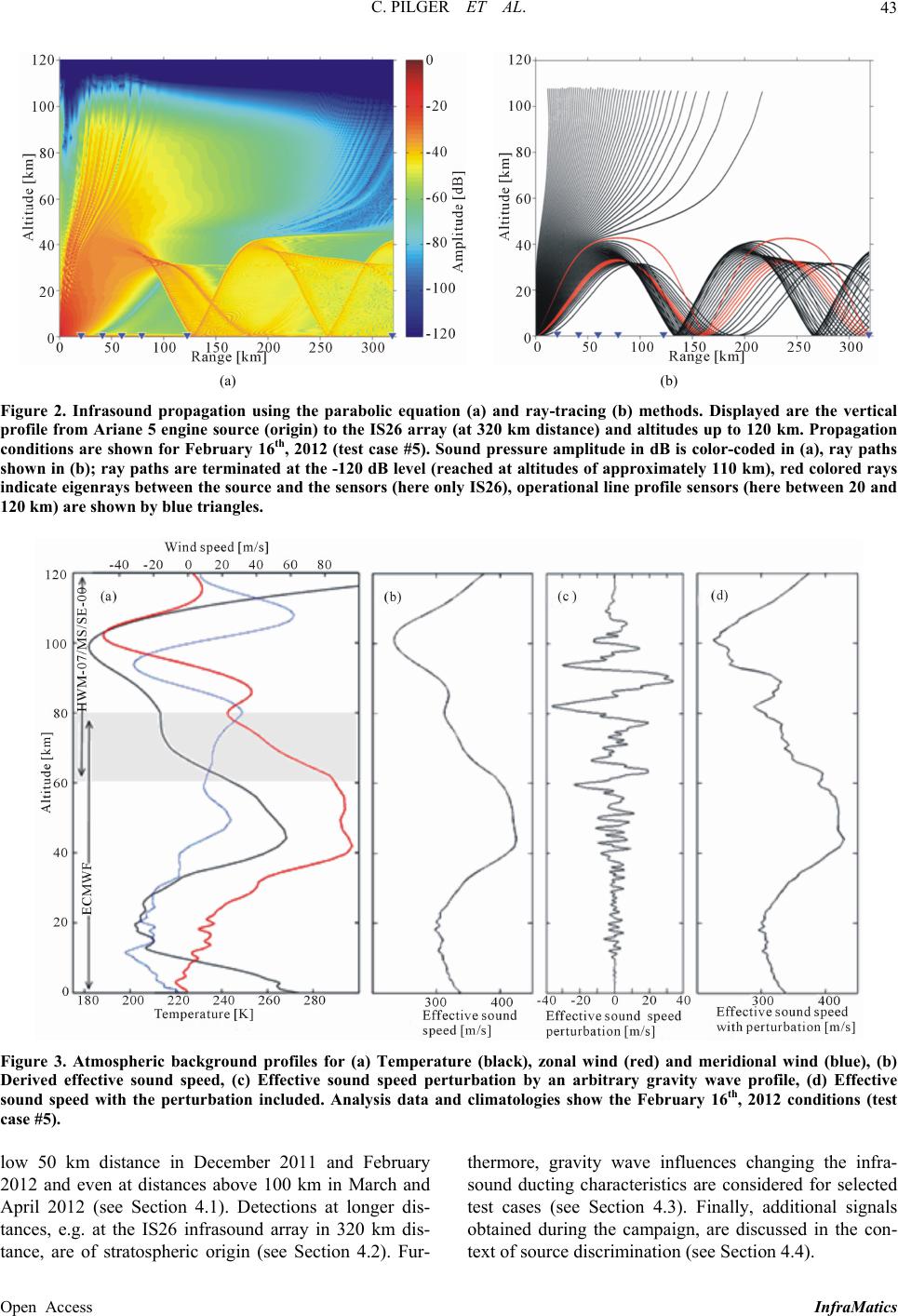

C. PILGER ET AL.

Open Access InfraMatics

(a) (b)

Figure 2. Infrasound propagation using the parabolic equation (a) and ray-tracing (b) methods. Displayed are the vertical

profile from Ariane 5 engine source (origin) to the IS26 array (at 320 km distance) and altitudes up to 120 km. Propagation

conditions are shown for February 16th, 2012 (test case #5). Sound pressure amplitude in dB is color-coded in (a), ray paths

shown in (b); ray paths are terminated at the -120 dB level (reached at altitudes of approximately 110 km), red colored rays

indicate eigenrays between the source and the sensors (here only IS26), operational line profile sensors (here between 20 and

120 km) are shown by blue triangles.

Figure 3. Atmospheric background profiles for (a) Temperature (black), zonal wind (red) and meridional wind (blue), (b)

Derived effective sound speed, (c) Effective sound speed perturbation by an arbitrary gravity wave profile, (d) Effective

sound speed with the perturbation included. Analysis data and climatologies show the February 16th, 2012 conditions (test

case #5).

low 50 km distance in December 2011 and February

2012 and even at distances above 100 km in March and

April 2012 (see Section 4.1). Detections at longer dis-

tances, e.g. at the IS26 infrasound array in 320 km dis-

tance, are of stratospheric origin (see Section 4.2). Fur-

thermore, gravity wave influences changing the infra-

sound ducting characteristics are considered for selected

test cases (see Section 4.3). Finally, additional signals

obtained during the campaign, are discussed in the con-

text of source discrimination (see Section 4.4).

C. PILGER ET AL.

4.1. Tropospheric Ducting

Detections of tropospheric arrivals were obtained in the

near-source shadow zone, where no stratospheric arrivals

are predicted, or in the case of April 2012 during a sea-

son, where only weak or more likely no stratospheric

ducting from west to east takes place. These detections

and their association to tropospheric ducting are in good

agreement with infrasound propagation modeling. Fur-

ther seismo-acoustic detections at 20 km distance (sta-

tion SIND) for test cases #1, #2, #3, #5, #6, and #8 and

non-detections for cases #4, #7, and #9 (see Table 1)

confirm the near-field infrasound measurements as well

as the modeling. In the following, a few specific exam-

ples of tropospheric ducting at regional distances are pre-

sented.

Figure 4(a) shows the results of propagation modeling

for the 19 December 2011 test case (#3). Infrasound de-

tections from this case were obtained at 40 and 320 km,

while sensors at 60, 80, 100, and 120 km had no detec-

tions. Figure 4(b) shows an enlarged view of the propa-

gation modeling at short distances, highlighting a tropo-

spheric duct. HARPA/DLR ray-trace modeling is su-

perimposed on the PE amplitude field in the figure, both

showing a tropospheric duct between the surface and an

altitude of a few 100 meters. In the ray-tracing, a number

of paths are observed that are each terminated when a limit

of ten surface reflections is reached. From this test case

and based on the observations and the modeling results,

it can be expected that a duct of only a few hundred me-

ters altitude cannot be observed beyond a maximum dis-

tance of 10 - 50 km distance, i.e. a maximum of 5 - 10

reflections. This is due to leaking of the sound energy

from the duct, especially when the infrasonic wavelength

is in the order of the vertical dimension of the duct and

when defocusing by topographic effects near the surface

[33] takes place. Unfortunately our PE modeling cannot

be used to study this scenario in detail, because the 1-D

version used here does not allow for inclusion of hori-

zontal variations of background conditions, orography or

near-surface attenuation. Therefore the tropospheric duct

is removed from the PE model cases in the following

considerations of stratospheric arrivals within Sections

4.2 and 4.3 of this paper. The line profile observations as

well as a seismo-acoustic detection at 20 km distance

(see Tab l e 1) are in good agreement with the model re-

sults based on the meteorological conditions at hand: a

layer of higher effective sound speed in approximately

400 m altitude above the surface, generating a tropo-

spheric duct. At distances larger than 40 km, no signals

from the tropospheric duct were found. The detection at

320 km is of stratospheric origin (see section 4.2). The

16 February 2012 test case (#5, see Figure 2) is very

similar to this case (with a seismo-acoustic and acoustic

detection at 20 km, no detections at 40, 60, and 80 km

and stratospheric detections at 120 km and 320 km), and

thus not further discussed here.

Figure 5(a) shows modeling results of the 16 January

2012 test case (#4). The same station-distance-setup is

used as for test case #5, but no detections were made

from 20 to 80 km distance. Detections at 120 and 320 km

are again from stratospheric paths and are discussed in

section 4.2. No tropospheric detections were identified

and modeling results hence do not show a tropospheric

duct. Figure 5(b) shows the same range-height-detail as

Figure 4(b) (blue triangles for stations at 20 and 40 km),

but the PE sound amplitude profile and HARPA/DLR

rays are strongly bending upwards. Meteorological con-

ditions cause a decreasing effective sound speed with

altitude in the first 10 kilometers and thus inhibit a tro-

pospheric duct, such that the lack of detections and the

modeling are again in good agreement.

A case of long distance tropospheric ducting is evi-

denced by the 27 April 2012 test case (#8). PE- and RT-

(a) (b)

Figure 4. Combined parabolic equation and ray-tracing profiles for the 19 December 2011 test case #3. (a) Complete propa-

gation path from Ariane 5 engine source to IS26 infr asound array . (b) Zoom of the first 50 km horizontal distance and 10 km

altitude highlighting a tropospheric duct. See Figure 2 for further details.

Open Access InfraMatics

C. PILGER ET AL. 45

(a) (b)

Figure 5. As Figure 4, but for the 16 January 2012 test case #4, with atmospheric conditions for which no tropospheric duct

was generated.

modeling shown in Figure 6(a) include a tropospheric

duct over the whole distance range which is persistent

between the surface and an altitude of 3 - 4 km. Since

this altitude is much higher than the few hundred meters

in cases #3 and #5, tropospheric ducting over large dis-

tances is theoretically possible at this altitude [14], as

disturbances due to orography and boundary layer turbu-

lence are strongly reduced. Signal measurements by sen-

sors at 120, 140, and 180 km were obtained and could be

attributed to tropospheric ducting: Figure 6(b) shows a

range versus travel-time plot for the ray-trace model,

where incidence points of rays at the surface are com-

pared to travel-times observed by the line profile sensors.

Observations between 120 and 180 km correspond to the

modeled tropospheric duct. Their celerity (range over

ground divided by travel-time) is about 350 m/s, which is

a fairly high value and thus indicates tropospheric duct-

ing (see [17,34]). However, the travel-time estimate for

the observation at 320 km distance is higher than ex-

pected for the tropospheric duct. The celerity of this de-

tection is about 300 m/s, which would be in a typical

range for stratospheric ducting [17,34], even though no

such duct is predicted by the modeling. Potential expla-

nations for this disagreement between modeling and

measurement will be given in Section 4.3. The detection

and corresponding modeling of a tropospheric duct

reaching out to 180 km from the source is a rare finding

which gives new insights into infrasound propagation at

regional distances.

4.2. Stratospheric Ducting & Amplitude

Estimations

Classical infrasound propagation from a surface source to

a sensor in some hundred kilometers distance is strongly

influenced by the stratospheric effective sound speed.

During atmospheric conditions, when the effective sound

speed in the stratosphere is higher than the effective

sound speed near the surface, stratospheric ducting takes

place and sound is (repeatedly) refracted from the strato-

sphere back to the surface. For infrasound propagation

from west to east, these conditions normally occur in

wintertime in the Northern Hemisphere (e.g. [26]). Since

most tests within this study took place during the winter

months, stratospheric arrivals at sensors installed at dis-

tances of more than 150 km were expected and regularly

observed. For certain test cases (e.g. #4, #5 and #7) with

extremely high vertical gradients of the effective sound

speed between 30 and 50 km altitude, stratospheric arri-

vals were already observed in 120 km distance from the

source. The zonal wind speed in test case #5 (see Figure

3) increases 70 - 80 m/s between altitudes of 30 - 40 km,

which can be associated, for example, with a strong jet

stream. Conditions in test cases #4 and #7 lead to similar

signal arrivals. Observations of signals in 120 km dis-

tance of the source and their arrival via stratosphere or

troposphere are discussed in the course of this section.

Comparisons between modeling results and measure-

ments were also performed with respect to infrasound

amplitudes. Amplitudes from modeling were estimated

using the surface level output from PE modeling as

sound pressure level in decibel (dB) at a reference range

of 1 km. For the comparison of these modeling ampli-

tudes with measurements in Pascal (Pa), a reference val-

ue for the source amplitude (in Pa at 1 km distance) to

equalize with 0 dB is needed.

Figure 7 shows a sound pressure level recording of the

last Ariane 5 engine test (#9) measured at 24 m distance

to the source. For a reference distance of 1 km, this sig-

nal of approximately 137 dB (corresponding to 142 Pa) is

reduced to a value between 120 dB (20 Pa) and 100 dB

(2 Pa) depending on the geometry assumptions for the

acoustic loss calculations [35]. Since different source and

propagation conditions may occur and thus different

Open Access InfraMatics

C. PILGER ET AL.

(a) (b)

Figure 6. (a) As Figure 4(a), but for the 27 April 2012 test case #8 and a tropospheric duct extending to an altitude of 3 - 4 km.

(b) Travel time estimation for all ray-tracing surface returns in the tropospheric duct (black dots) and onset-times derived

from observations (red crosses) in sensor distances (blue lines).

Figure 7. Sound pressure level measurement performed in

the audible range during the 14 May 2012 test #9 at a dis-

tance of 24 m to the Ariane 5 engine. The sound pressure

level is increased for the test duration of 530 s from 70 dB

ambient noise (which is already an increased value due to

background noise before and after the test, compared to

usually 30 - 50 dB) to about 137 dB during the engine test.

sound pressure levels for different test cases may result,

an intermediate value of 10 Pa source amplitude (at 1 km)

is chosen corresponding then to 0 dB modeling ampli-

tude.

Figure 8 shows comparisons of modeled amplitude

values derived using the surface level values from the PE

method and observed signal amplitudes for the test cases

#3, #4 and #5 (already discussed for tropospheric ducting

in section 4.1; propagation diagrams for these cases are

shown in Figures 2, 4 and 5). Amplitudes derived from

modeling and observations are in good agreement and

show stratospheric detections at IS26 (at 320 km). Fur-

thermore, stratospheric ducting beginning at 120 km dis-

tance explains detections in cases #4 and #5 (January and

February) but not in case #3 (December). A beginning

stratospheric duct at 120 +/− 5 km in the model explains

the January and February detections, whereas in Decem-

ber, due to the atmospheric conditions, stratospheric

ducting sets in at 150 +/− 5 km, which is in good agree-

ment with the lack of a stratospheric arrival at 120 km in

that case.

For cases #3 and #5 (and #6 in Figure 9), tropospheric

(dotted curves) and stratospheric ducting (dashed curves)

were modeled separately. Since the used PE method only

allowed one-dimensional background conditions, a tro-

pospheric duct does not fade over the modeling distance.

However, both observations and ray-tracing show that

the tropospheric ducts vanishes beyond the first observa-

tion point and thus the two ducting regimes were com-

bined in these cases by merging the profiles (solid lines)

and applying a linear transition from tropospheric to

stratospheric ducting.

The root mean square (RMS) deviation was calculated

as a measure to quantify the difference/agreement be-

tween observations and modeling. For the abovemen-

tioned cases, results are 3.26 dB (case #3), 8.27 dB (case

#4) and 25.07 dB (case #5), which corresponds to devia-

tions of about one order of pressure magnitude. However,

only two to three detections were available for these cas-

es and conclusions on the estimation of amplitudes from

this should be drawn with caution.

More specific examples with observations by six sen-

sors are the March 7 and March 22, 2012 Ariane test

cases #6 and #7 shown in Figures 9 and 10, describing

stratospheric duct modeling and corresponding observa-

tions in greater detail.

In test case #6, stratospheric ducting of the engine test

signal is observed at distances of 160, 180, 210, and 240

km as well as IS26 in 320 km. Modeling of the first and

second stratospheric return to the surface (see Figure

9(a)) explains most of these observations. Only the ob-

servation at the first sensor in 120 km distance cannot be

explained by stratospheric ducting and is (similar to case

#8, see Figure 6) of tropospheric origin. Infrasonic travel

Open Access InfraMatics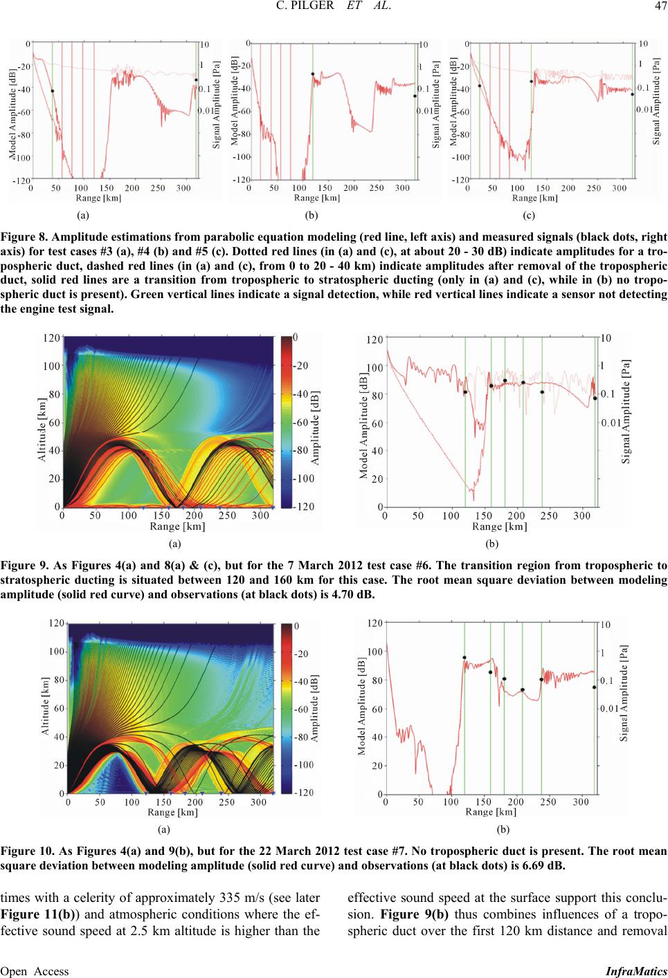

C. PILGER ET AL. 47

(a) (b) (c)

Figure 8. Amplitude e stimations from parabolic equation modeling (red line, left axis) and measured signals (black dots, right

axis) for test cases #3 (a), #4 (b) and #5 (c). Dotted red lines (in (a) and (c), at about 20 - 30 dB) indicate amplitudes for a tro-

pospheric duct, dashed red lines (in (a) and (c), from 0 to 20 - 40 km) indicate amplitudes after removal of the tropospheric

duct, solid red lines are a transition from tropospheric to stratospheric ducting (only in (a) and (c), while in (b) no tropo-

spheric duct is present). Green vertical lines indicate a signal detection, while red ver tical lines indicate a sensor not dete cting

the engine test signal.

(a) (b)

Figure 9. As Figures 4(a) and 8(a) & (c), but for the 7 March 2012 test case #6. The transition region from tropospheric to

stratospheric ducting is situated between 120 and 160 km for this case. The root mean square deviation between modeling

amplitude (solid red curve) and observations (at black dots) is 4.70 dB.

(a) (b)

Figure 10. As Figures 4(a) and 9(b), but for the 22 March 2012 test case #7. No tropospheric duct is present. The root mean

square deviation betw ee n mode ling amplitude (solid red curve) and observations (at black dots) is 6.69 dB.

times with a celerity of approximately 335 m/s (see later

Figure 11(b)) and atmospheric conditions where the ef-

fective sound speed at 2.5 km altitude is higher than the

effective sound speed at the surface support this conclu-

sion. Figure 9(b) thus combines influences of a tropo-

spheric duct over the first 120 km distance and removal

Open Access InfraMatics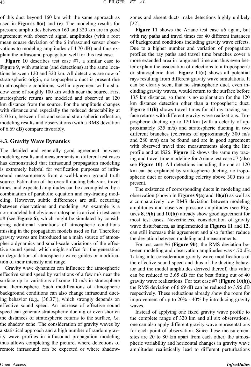

C. PILGER ET AL.

of this duct beyond 160 km with the same approach as

used in Figures 8(a) and (c). The modeling results for

pressure amplitudes between 160 and 320 km are in good

agreement with observed signal amplitudes (with a root

mean square deviation of the 6 infrasound sensor obser-

vations to modeling amplitudes of 4.70 dB) and thus ex-

plain the infrasound propagation well for this test case.

Figure 10 describes test case #7, a similar case to

Figure 9, with stations (and detections) at the same loca-

tions between 120 and 320 km. All detections are now of

stratospheric origin, no tropospheric duct is present due

to atmospheric conditions, well in agreement with a sha-

dow zone of roughly 100 km width near the source. First

stratospheric returns are modeled and observed at 120

km distance from the source. For the amplitude changes

with distance and especially the reduced detectability at

210 km, between first and second stratospheric reflection,

modeling results and observations (with a RMS deviation

of 6.69 dB) compare favorably.

4.3. Gravity Wave Dynamics

The detailed and generally good agreement between

modeling results and measurements in different test cases

has demonstrated that infrasound propagation modeling

is extremely helpful for verification purposes of infra-

sound measurements from a well-known ground truth

source. Estimation of the overall ducting behavior, travel

times, and expected amplitudes can be accomplished by a

combination of parabolic equation and ray-tracing mod-

eling. However, subtle differences are still occurring

between observations and modeling. An example is a

non-modeled but obvious stratospheric arrival in test case

#8 (see Figure 6), which might be simulated by consid-

ering additional variations of atmospheric conditions

missing in the propagation models used so far. Therefore

gravity waves are introduced as a main source of atmos-

pheric dynamics and small-scale variations of the effec-

tive sound speed, which might suffice for the generation

or degradation of atmospheric wave guides or modifica-

tion of their intensity and range.

Gravity wave dynamics can influence the atmospheric

effective sound speed by variations of a few m/s near the

surface up to variations of some 10 m/s in stratosphere

and thermosphere. Such modifications of atmospheric

background conditions can also change infrasound duct-

ing behavior (e.g., [36,37]), which strongly depends on

effective sound speed. An increase of effective sound

speed can generate stratospheric ducting or even shorten

the distances of stratospheric returns to the surface, i.e.

the shadow zone. The consideration of gravity waves by

a statistical approach and a high number of random grav-

ity wave profiles in infrasound propagation modeling

thus allows completing the picture, where detections of

remote infrasound can be expected or where shadow-

zones and absent ducts make detections highly unlikely

[22].

Figure 11 shows the Ariane test case #6 again, but

with ray paths and travel times for 40 different instances

of background conditions including gravity wave effects.

Due to a higher number and variation of propagation

profiles the ray paths and travel time branches cover a

more extended area in range and time and thus even bet-

ter explain the association of detections to a tropospheric

or stratospheric duct. Figure 11(a) shows all potential

rays resulting from different gravity wave simulations. It

can be clearly seen, that no stratospheric duct, even in-

cluding gravity waves, would return to the surface before

135 km distance, so there is no explanation for the 120

km distance detection other than a tropospheric duct.

Figure 11(b) shows travel times for all ray tracing sur-

face returns with different gravity wave realizations. Tro-

pospheric ducting up to 120 km (with a celerity of ap-

proximately 335 m/s) and stratospheric ducting in two

different branches (celerities of approximately 300 m/s

and 280 m/s) can be found and are in good agreement

with observed travel time measurements along the line

profile and at IS26. Figure 12 shows the same ray trac-

ing and travel time modeling for Ariane test case #7 (also

see Figure 10). All detections including the one at 120

km can be explained by stratospheric ducting, no tropo-

spheric duct or corresponding celerity above 300 m/s is

present.

The existence of corresponding ducts in modeling and

observation (shown in Figures 9(a) and 10(a)) as well as

a comparatively low RMS deviation between modeling

amplitudes and observed pressure amplitudes (see Fig-

ures 8, 9(b) and 10(b)) already show good agreement for

most test cases. Nevertheless, consideration of gravity

wave disturbances, as implemented in Figures 11 and 12,

can still increase this agreement and also further reduce

the deviation between modeling and measurements.

For test case #6 (Figure 9b), the RMS deviation be-

tween modeling and observation amplitudes was 4.70 dB.

Taking into consideration gravity wave modifications of

the effective sound speed and thus of the ducting behav-

ior and the model amplitudes derived thereof, this value

can be reduced to 3.65 dB for the best fitting out of 40

gravity wave realizations. For test case #7 (Figure 10(b)),

the RMS deviation of 6.69 dB can be reduced to 3.96 dB

respectively. These reductions already show the room for

improvement of up to 20% - 40% by introducing gravity

waves.

Instead of applying one fixed gravity wave profile to

the complete range of 320 km and all six observations,

one can also apply different gravity wave representations

for each point of observation. Since these measurement

sites are 20 to 80 km apart from each other, the atmos-

pheric variability and horizontal changes in gravity wave

amplitudes realistically lead to different perturbations

Open Access InfraMatics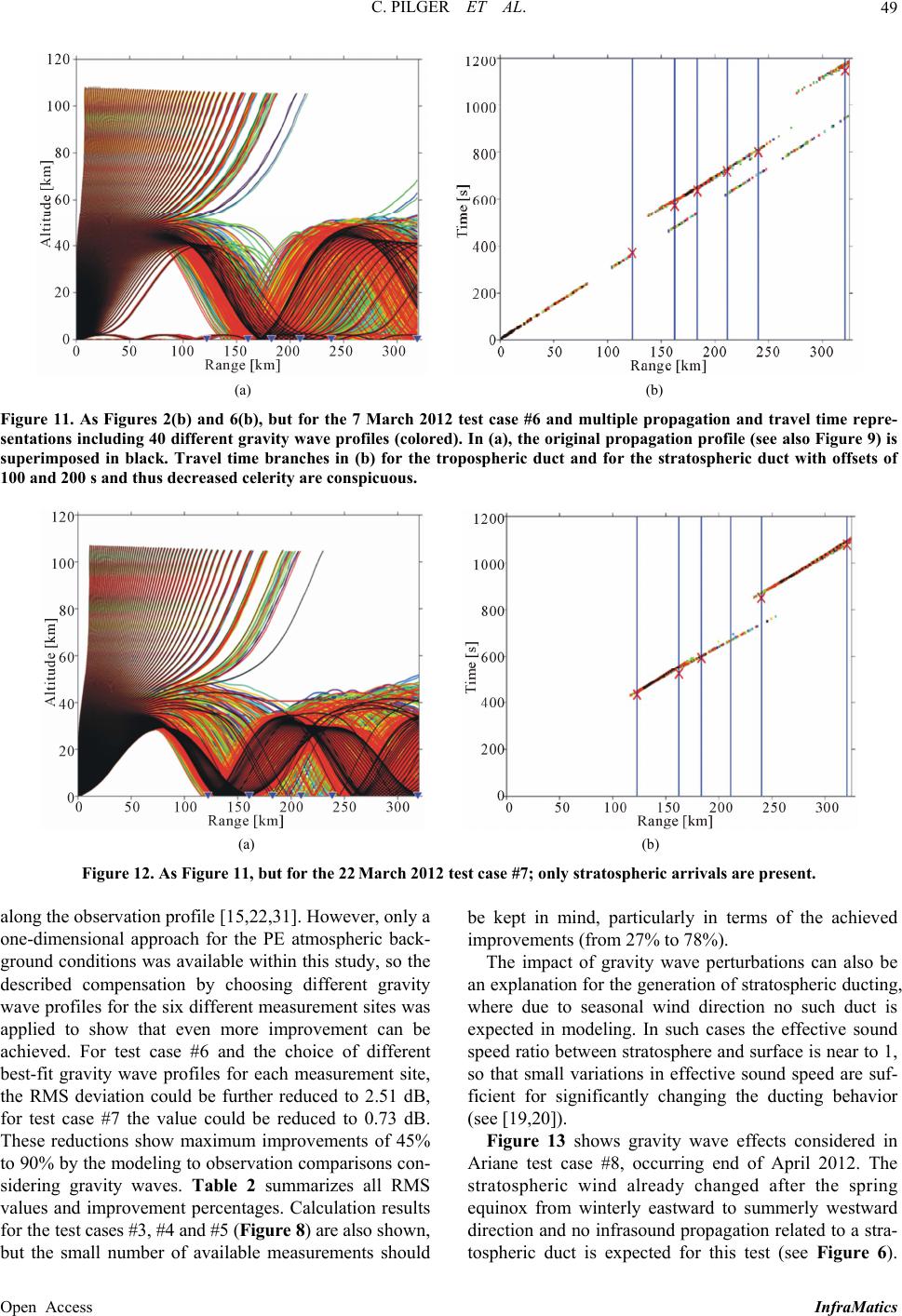

C. PILGER ET AL.

Open Access InfraMatics

(a) (b)

Figure 11. As Figures 2(b) and 6(b), but for the 7 March 2012 test case #6 and multiple propagation and travel time repre-

sentations including 40 different gravity wave profiles (colored). In (a), the original propagation profile (see also Figure 9) is

superimposed in black. Travel time branches in (b) for the tropospheric duct and for the stratospheric duct with offsets of

100 and 200 s and thus decreased celerity are conspicuous.

(a) (b)

Figure 12. As Figure 11, but for the 22 March 2012 test case #7; only stratospheric arrivals are present.

along the observation profile [15,22,31]. However, only a

one-dimensional approach for the PE atmospheric back-

ground conditions was available within this study, so the

described compensation by choosing different gravity

wave profiles for the six different measurement sites was

applied to show that even more improvement can be

achieved. For test case #6 and the choice of different

best-fit gravity wave profiles for each measurement site,

the RMS deviation could be further reduced to 2.51 dB,

for test case #7 the value could be reduced to 0.73 dB.

These reductions show maximum improvements of 45%

to 90% by the modeling to observation comparisons con-

sidering gravity waves. Table 2 summarizes all RMS

values and improvement percentages. Calculation results

for the test cases #3, #4 and #5 (Figure 8) are also shown,

but the small number of available measurements should

be kept in mind, particularly in terms of the achieved

improvements (from 27% to 78%).

The impact of gravity wave perturbations can also be

an explanation for the generation of stratospheric ducting,

where due to seasonal wind direction no such duct is

expected in modeling. In such cases the effective sound

speed ratio between stratosphere and surface is near to 1,

so that small variations in effective sound speed are suf-

ficient for significantly changing the ducting behavior

(see [19,20]).

Figure 13 shows gravity wave effects considered in

Ariane test case #8, occurring end of April 2012. The

stratospheric wind already changed after the spring

equinox from winterly eastward to summerly westward

direction and no infrasound propagation related to a stra-

tospheric duct is expected for this test (see Figure 6).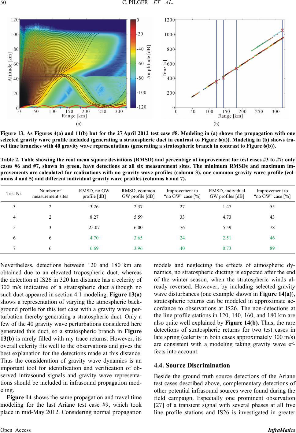

C. PILGER ET AL.

(a) (b)

Figure 13. As Figures 4(a) and 11(b) but for the 27 April 2012 test case #8. Modeling in (a) shows the propagation with one

selected gravity wave profile included (generating a stratospheric duct in contrast to Figure 6(a)). Modeling in (b) shows tra-

vel time branches with 40 gravity wave representations (generating a stratospheric branch in contrast to Figure 6(b)).

Table 2. Table showing the root mean square deviations (RMSD) and percentage of improvement for test cases #3 to #7; only

cases #6 and #7, shown in green, have detections at all six measurement sites. The minimum RMSDs and maximum im-

provements are calculated for realizations with no gravity wave profiles (column 3), one common gravity wave profile (col-

umns 4 and 5) and different individual gravity wave profiles (columns 6 and 7).

Test Nr. Number of

measurement sites

RMSD, no GW

profile [dB]

RMSD, common

GW profile [dB]

Improvement to

“no GW” case [%]

RMSD, individual

GW profiles [dB]

Improvement to

“no GW” case [%]

3 2 3.26 2.37 27 1.47 55

4 2 8.27 5.59 33 4.73 43

5 3 25.07 6.00 76 5.59 78

6 6 4.70 3.65 24 2.51 46

7 6 6.69 3.96 40 0.73 89

Nevertheless, detections between 120 and 180 km are

obtained due to an elevated tropospheric duct, whereas

the detection at IS26 in 320 km distance has a celerity of

300 m/s indicative of a stratospheric duct although no

such duct appeared in section 4.1 modeling. Figure 13(a)

shows a representation of varying the atmospheric back-

ground profile for this test case with a gravity wave per-

turbation thereby generating a stratospheric duct. Only a

few of the 40 gravity wave perturbations considered here

generated this duct, so a stratospheric branch in Figure

13(b) is rarely filled with ray trace returns. However, its

overall celerity fits well to the observations and gives the

best explanation for the detections made at this distance.

Thus the consideration of gravity wave dynamics is an

important tool for identification and verification of ob-

served infrasound signals and gravity wave representa-

tions should be included in infrasound propagation mod-

eling.

Figure 14 shows the same propagation and travel time

modeling for the last Ariane test case #9, which took

place in mid-May 2012. Considering normal propagation

models and neglecting the effects of atmospheric dy-

namics, no stratospheric ducting is expected after the end

of the winter season, when the stratospheric winds al-

ready reversed. However, by including selected gravity

wave disturbances (one example shown in Figure 14(a)),

stratospheric returns can be modeled in approximate ac-

cordance to observations at IS26. The non-detections at

the line profile stations in 120, 140, 160, and 180 km are

also quite well explained by Figure 14(b). Thus, the rare

detections of stratospheric returns for two test cases in

late spring (celerity in both cases approximately 300 m/s)

are consistent with a modeling taking gravity wave ef-

fects into account.

4.4. Source Discrimination

Beside the ground truth source detections of the Ariane

test cases described above, complementary detections of

other potential infrasound sources were found during the

field campaign. Especially one prominent observation

[27] of a transient signal with several phases at all five

line profile stations and IS26 is investigated in greater

Open Access InfraMatics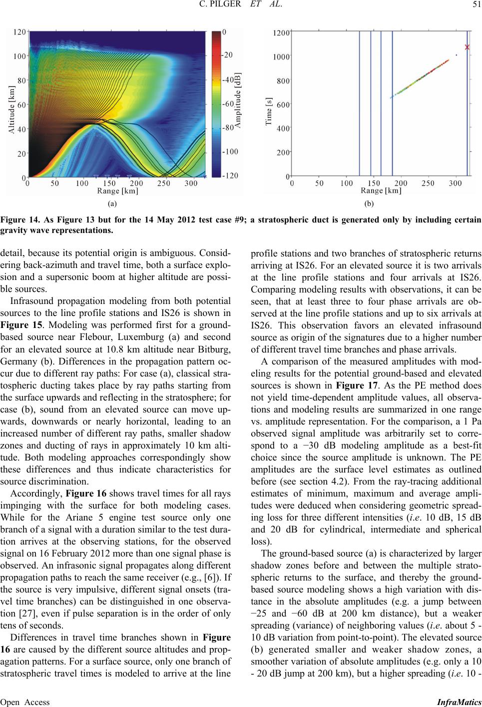

C. PILGER ET AL. 51

(a) (b)

Figure 14. As Figure 13 but for the 14 May 2012 test case #9; a stratospheric duct is generated only by including certain

gravity wave representations.

detail, because its potential origin is ambiguous. Consid-

ering back-azimuth and travel time, both a surface explo-

sion and a supersonic boom at higher altitude are possi-

ble sources.

Infrasound propagation modeling from both potential

sources to the line profile stations and IS26 is shown in

Figure 15. Modeling was performed first for a ground-

based source near Flebour, Luxemburg (a) and second

for an elevated source at 10.8 km altitude near Bitburg,

Germany (b). Differences in the propagation pattern oc-

cur due to different ray paths: For case (a), classical stra-

tospheric ducting takes place by ray paths starting from

the surface upwards and reflecting in the stratosphere; for

case (b), sound from an elevated source can move up-

wards, downwards or nearly horizontal, leading to an

increased number of different ray paths, smaller shadow

zones and ducting of rays in approximately 10 km alti-

tude. Both modeling approaches correspondingly show

these differences and thus indicate characteristics for

source discrimination.

Accordingly, Figure 16 shows travel times for all rays

impinging with the surface for both modeling cases.

While for the Ariane 5 engine test source only one

branch of a signal with a duration similar to the test dura-

tion arrives at the observing stations, for the observed

signal on 16 February 2012 more than one signal phase is

observed. An infrasonic signal propagates along different

propagation paths to reach the same receiver (e.g., [6]). If

the source is very impulsive, different signal onsets (tra-

vel time branches) can be distinguished in one observa-

tion [27], even if pulse separation is in the order of only

tens of seconds.

Differences in travel time branches shown in Figure

16 are caused by the different source altitudes and prop-

agation patterns. For a surface source, only one branch of

stratospheric travel times is modeled to arrive at the line

profile stations and two branches of stratospheric returns

arriving at IS26. For an elevated source it is two arrivals

at the line profile stations and four arrivals at IS26.

Comparing modeling results with observations, it can be

seen, that at least three to four phase arrivals are ob-

served at the line profile stations and up to six arrivals at

IS26. This observation favors an elevated infrasound

source as origin of the signatures due to a higher number

of different travel time branches and phase arrivals.

A comparison of the measured amplitudes with mod-

eling results for the potential ground-based and elevated

sources is shown in Figure 17. As the PE method does

not yield time-dependent amplitude values, all observa-

tions and modeling results are summarized in one range

vs. amplitude representation. For the comparison, a 1 Pa

observed signal amplitude was arbitrarily set to corre-

spond to a −30 dB modeling amplitude as a best-fit

choice since the source amplitude is unknown. The PE

amplitudes are the surface level estimates as outlined

before (see section 4.2). From the ray-tracing additional

estimates of minimum, maximum and average ampli-

tudes were deduced when considering geometric spread-

ing loss for three different intensities (i.e. 10 dB, 15 dB

and 20 dB for cylindrical, intermediate and spherical

loss).

The ground-based source (a) is characterized by larger

shadow zones before and between the multiple strato-

spheric returns to the surface, and thereby the ground-

based source modeling shows a high variation with dis-

tance in the absolute amplitudes (e.g. a jump between

−25 and −60 dB at 200 km distance), but a weaker

spreading (variance) of neighboring values (i.e. about 5 -

10 dB variation from point-to-point). The elevated source

(b) generated smaller and weaker shadow zones, a

smoother variation of absolute amplitudes (e.g. only a 10

- 20 dB jump at 200 km), but a higher spreading (i.e. 10 -

Open Access InfraMatics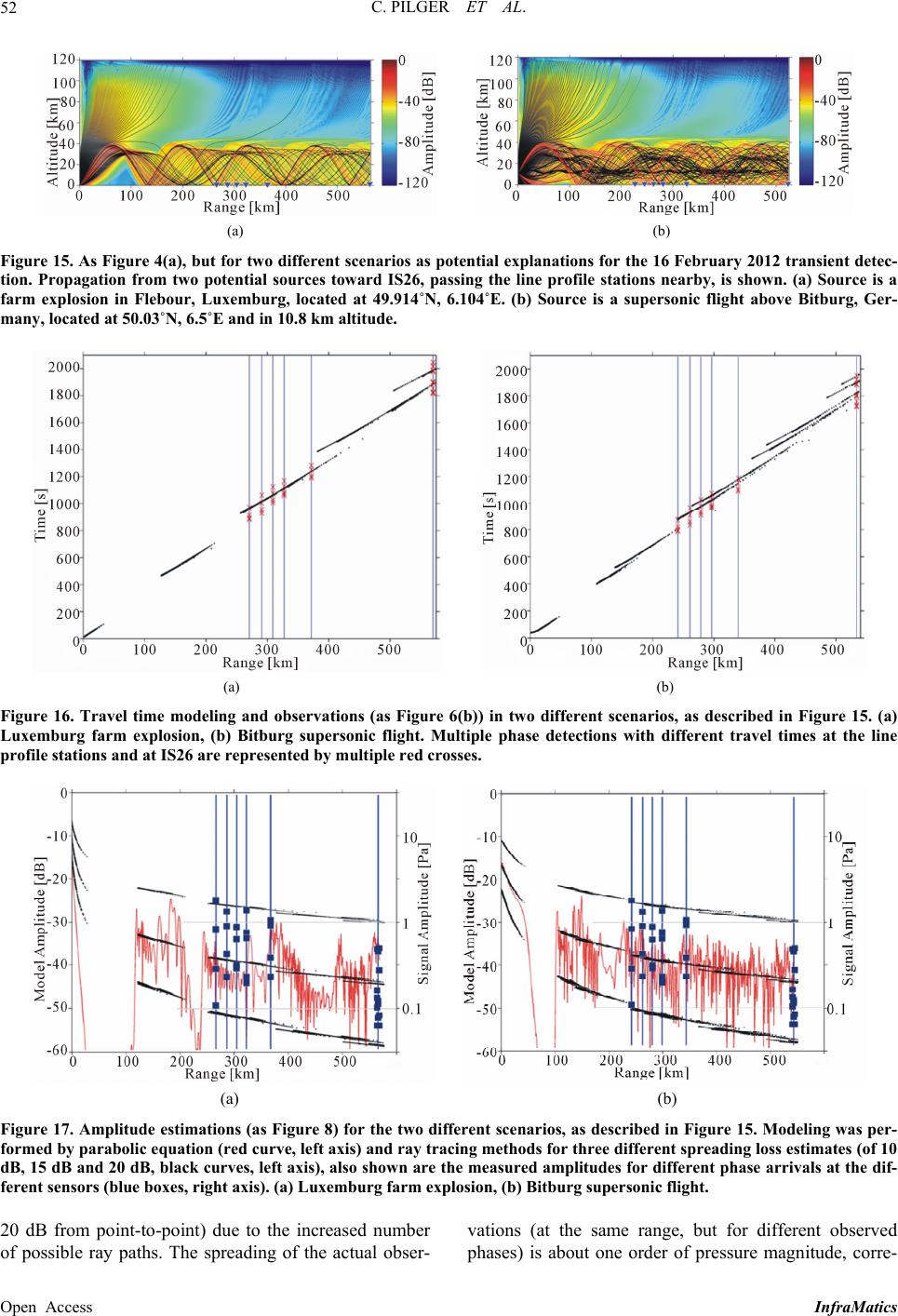

C. PILGER ET AL.

(a) (b)

Figure 15. As Figure 4(a), but for two different scenarios as potential explanations for the 16 February 2012 transient detec-

tion. Propagation from two potential sources toward IS26, passing the line profile stations nearby, is shown. (a) Source is a

farm explosion in Flebour, Luxemburg, located at 49.914˚N, 6.104˚E. (b) Source is a supersonic flight above Bitburg, Ger-

many, located at 50.03˚N, 6.5˚E and in 10.8 km altitude.

(a) (b)

Figure 16. Travel time modeling and observations (as Figure 6(b)) in two different scenarios, as described in Figure 15. (a)

Luxemburg farm explosion, (b) Bitburg supersonic flight. Multiple phase detections with different travel times at the line

profile stations and at IS26 are represented by multiple red crosses.

(a) (b)

Figure 17. Amplitude estimations (as Figure 8) for the two different scenarios, as described in Figure 15. Modeling was per-

formed by parabolic equation (red curve, left axis) and ray tracing methods for three different spreading loss estimates (of 10

dB, 15 dB and 20 dB, black curves, left axis), also shown are the measured amplitudes for different phase arri vals at the dif-

ferent sensors (blue boxes, right axis). (a) Luxemburg farm explosion, (b) Bitburg supersonic flight.

20 dB from point-to-point) due to the increased number

of possible ray paths. The spreading of the actual obser-

vations (at the same range, but for different observed

phases) is about one order of pressure magnitude, corre-

Open Access InfraMatics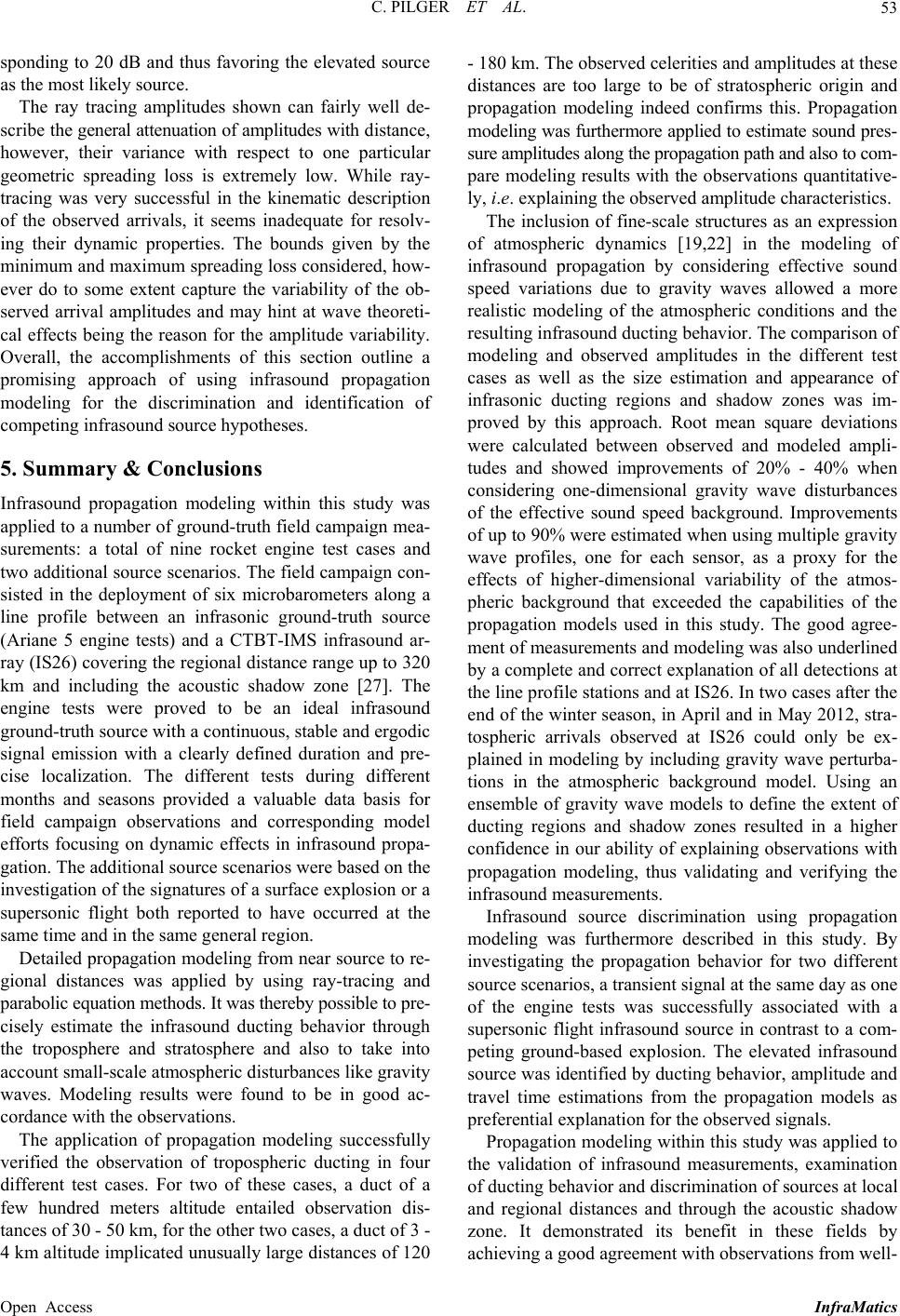

C. PILGER ET AL. 53

sponding to 20 dB and thus favoring the elevated source

as the most likely source.

The ray tracing amplitudes shown can fairly well de-

scribe the general attenuation of amplitudes with distance,

however, their variance with respect to one particular

geometric spreading loss is extremely low. While ray-

tracing was very successful in the kinematic description

of the observed arrivals, it seems inadequate for resolv-

ing their dynamic properties. The bounds given by the

minimum and maximum spreading loss considered, how-

ever do to some extent capture the variability of the ob-

served arrival amplitudes and may hint at wave theoreti-

cal effects being the reason for the amplitude variability.

Overall, the accomplishments of this section outline a

promising approach of using infrasound propagation

modeling for the discrimination and identification of

competing infrasound source hypotheses.

5. Summary & Conclusions

Infrasound propagation modeling within this study was

applied to a number of ground-truth field campaign mea-

surements: a total of nine rocket engine test cases and

two additional source scenarios. The field campaign con-

sisted in the deployment of six microbarometers along a

line profile between an infrasonic ground-truth source

(Ariane 5 engine tests) and a CTBT-IMS infrasound ar-

ray (IS26) covering the regional distance range up to 320

km and including the acoustic shadow zone [27]. The

engine tests were proved to be an ideal infrasound

ground-truth source with a continuous, stable and ergodic

signal emission with a clearly defined duration and pre-

cise localization. The different tests during different

months and seasons provided a valuable data basis for

field campaign observations and corresponding model

efforts focusing on dynamic effects in infrasound propa-

gation. The additional source scenarios were based on the

investigation of the signatures of a surface explosion or a

supersonic flight both reported to have occurred at the

same time and in the same general region.

Detailed propagation modeling from near source to re-

gional distances was applied by using ray-tracing and

parabolic equation methods. It was thereby possible to pre-

cisely estimate the infrasound ducting behavior through

the troposphere and stratosphere and also to take into

account small-scale atmospheric disturbances like gravity

waves. Modeling results were found to be in good ac-

cordance with the observations.

The application of propagation modeling successfully

verified the observation of tropospheric ducting in four

different test cases. For two of these cases, a duct of a

few hundred meters altitude entailed observation dis-

tances of 30 - 50 km, for the other two cases, a duct of 3 -

4 km altitude implicated unusually large distances of 120

- 180 km. The observed celerities and amplitudes at these

distances are too large to be of stratospheric origin and

propagation modeling indeed confirms this. Propagation

modeling was furthermore applied to estimate sound pres-

sure amplitudes along the propagation path and also to com-

pare modeling results with the observations quantitative-

ly, i.e. explaining the observed amplitude characteristics.

The inclusion of fine-scale structures as an expression

of atmospheric dynamics [19,22] in the modeling of

infrasound propagation by considering effective sound

speed variations due to gravity waves allowed a more

realistic modeling of the atmospheric conditions and the

resulting infrasound ducting behavior. The comparison of

modeling and observed amplitudes in the different test

cases as well as the size estimation and appearance of

infrasonic ducting regions and shadow zones was im-

proved by this approach. Root mean square deviations

were calculated between observed and modeled ampli-

tudes and showed improvements of 20% - 40% when

considering one-dimensional gravity wave disturbances

of the effective sound speed background. Improvements

of up to 90% were estimated when using multiple gravity

wave profiles, one for each sensor, as a proxy for the

effects of higher-dimensional variability of the atmos-

pheric background that exceeded the capabilities of the

propagation models used in this study. The good agree-

ment of measurements and modeling was also underlined

by a complete and correct explanation of all detections at

the line profile stations and at IS26. In two cases after the

end of the winter season, in April and in May 2012, stra-

tospheric arrivals observed at IS26 could only be ex-

plained in modeling by including gravity wave perturba-

tions in the atmospheric background model. Using an

ensemble of gravity wave models to define the extent of

ducting regions and shadow zones resulted in a higher

confidence in our ability of explaining observations with

propagation modeling, thus validating and verifying the

infrasound measurements.

Infrasound source discrimination using propagation

modeling was furthermore described in this study. By

investigating the propagation behavior for two different

source scenarios, a transient signal at the same day as one

of the engine tests was successfully associated with a

supersonic flight infrasound source in contrast to a com-

peting ground-based explosion. The elevated infrasound

source was identified by ducting behavior, amplitude and

travel time estimations from the propagation models as

preferential explanation for the observed signals.

Propagation modeling within this study was applied to

the validation of infrasound measurements, examination

of ducting behavior and discrimination of sources at local

and regional distances and through the acoustic shadow

zone. It demonstrated its benefit in these fields by

achieving a good agreement with observations from well-

Open Access InfraMatics

C. PILGER ET AL.

constrained ground-truth sources. By describing atmos-

pheric background conditions with high resolution, in-

cluding fine-scale variations by an ensemble of gravity

waves, even observations not expected from the standard

model could be well explained and the realistic state of

the atmosphere could be well represented by the ap-

proach followed within this study.

Further investigations combining propagation model-

ing with infrasound observations should include the rep-

resentation of multi-dimensional background conditions

in state of the art propagation models at high spatial and

temporal resolution, consideration of small-scale influ-

ences due to e.g. orography and near surface irregulari-

ties as well as an increased representation and under-

standing of gravity waves and their influence on atmos-

pheric dynamics. Results of such studies are invaluable

for improving infrasound detection capabilities, atmos-

pheric models and the understanding of infrasound proc-

esses on different scales.

6. Acknowledgements

We thank the counterpart from German Aerospace Center

Lampoldshausen (DLR-RA), the colleagues from the State

Seismological Survey of Baden-Württemberg (LEDBW),

and the German Airforce (Bundeswehr, Luftwaffenamt,

Flugbetriebs-und Informationszentrale, FLIZ) for provid-

ing information, data and support to this study.

We are grateful to Edgar Wetzig and Uwe Stelling for

their support in installing and maintaining the mobile

infrasound stations during the field campaign.

This work was partly performed in the course of the

ARISE collaborative project within the Seventh Frame-

work Programme funded by the European Union

(http://arise-project.eu/).

REFERENCES

[1] R. Matoza, J. Vergoz, A. Le Pichon, L. Ceranna, D. N.

Green, L. G. Evers, M. Ripepe, P. Campus, L. Liszka, T.

Kvaerna, E. Kjartansson and A. Höskuldsson, “Long-

Range Acoustic Observations of the Eyjafjallajökull Erup-

tion, Iceland, April-May 2010,” Geophysical Research

Letters, Vol. 38, No. 6, 2011, Article ID: L06308.

http://dx.doi.org/10.1029/2011GL047019

[2] D. Tailpied, A. Le Pichon, E. Marchetti, M. Ripepe, M.

Kallel and L. Ceranna, “Remote Infrasound Monitoring

of Mount Etna: Observed and Predicted Network Detec-

tion Capability,” InfraMatics, Vol. 2, No. 1, 2013, pp. 1-

11. http://dx.doi.org/10.4236/inframatics.2013.21001

[3] A. Le Pichon, L. Ceranna, C. Pilger, P. Mialle, D. Brown,

P. Herry and N. Brachet, “The 2013 Russian Fireball

Largest Ever Detected by CTBTO Infrasound Sensors,”

Geophysical Research Letters, Vol. 40, No. 14, 2013, pp.

3732-3736. http://dx.doi.org/10.1002/grl.50619

[4] C. D. de Groot-Hedlin, M. A. H. Hedlin, K. T. Walker, D.

P. Drob and M. A. Zumberge, “Evaluation of Infrasound

Signals from the Shuttle Atlantis Using a Large Seismic

Network,” Journal of the Acoustical Society of America,

Vol. 124, No. 3, 2008, pp. 1442-1451.

http://dx.doi.org/10.1121/1.2956475

[5] L. Ottemöller and L. G. Evers, “Seismo-Acoustic Analy-

sis of the Buncefield Oil Depot Explosion in the UK,

2005 December 11,” Geophysical Journal International,

Vol. 172, No. 3, 2008, pp. 1123-1134.

http://dx.doi.org/10.1111/j.1365-246X.2007.03701.x

[6] L. Ceranna, A. Le Pichon, D. N. Green and P. Mialle,

“The Buncefield Explosion: A Benchmark for Infrasound

Analysis across Central Europe,” Geophysical Journal

International, Vol. 177, No. 2, 2009, pp. 491-508.

http://dx.doi.org/10.1111/j.1365-246X.2008.03998.x

[7] P. Campus, “The IMS Infrasound Network and Its Poten-

tial for Detection of Events: Examples of a Variety of

Signals Recorded around the World,” InfraMatics, Vol. 6,

No. 1, 2004, pp. 13-22.

[8] A. Le Pichon, E. Blanc and A. Hauchecorne, “Infrasound

Monitoring for Atmospheric Studies,” Springer, Berlin,

2010.

[9] M. A. H. Hedlin, K. T. Walker, D. P. Drob and C. D. de

Groot-Hedlin, “Infrasound: Connecting the Solid Earth,

Oceans, and Atmosphere,” Annual Review of Earth and

Planetary Sciences, Vol. 40, 2012, pp. 327-254.

http://dx.doi.org/10.1146/annurev-earth-042711-105508

[10] M. A. Garces, “On Infrasound Standards, Part 1: Time,

Frequency, and Energy Scaling,” InfraMatics, Vol. 2, No.

2, 2013, pp. 13-35.

http://dx.doi.org/10.4236/inframatics.2013.22002

[11] A. Le Pichon, E. Blanc and D. P. Drob, “Probing High-

Altitude Winds Using Infrasound,” Journal of Geophysi-

cal Research, Vol. 110, No. D20, 2005, Article ID:

D20104.

[12] D. P. Drob, R. R. Meier, J. M. Picone and M. A. Garces,

“Inversion of Infrasound Signals for Passive Atmospheric

Remote Sensing,” In: A. Le Pichon, E. Blanc, and A.

Hauchecorne, Eds., Infrasound Monitoring for Atmos-

pheric Studies, Springer, Berlin, 2010.

http://dx.doi.org/10.1007/978-1-4020-9508-5_24

[13] J.-M. Lalande, O. Sèbe, M. Landès, P. Blanc-Benon, R. S.

Matoza, A. Le Pichon and E. Blanc, “Infrasound Data

Inversion for Atmospheric Sounding,” Geophysical Jour-

nal Internationa, Vol. 190, No. 1, 2012, pp. 687-701.

http://dx.doi.org/10.1111/j.1365-246X.2012.05518.x

[14] D. P. Drob, J. M. Picone and M. A. Garces, “Global Mor-

phology of Infrasound Propagation,” Journal of Geo-

physical Research, Vol. 108, No. D21, 2003, p. 4680.

[15] D. Norris and R. Gibson, “Numerical Methods to Model

Infrasound Propagation through Realistic Specifications

of the Atmosphere,” In: A. Le Pichon, E. Blanc and A.

Hauchecorne, Eds., Infrasound Monitoring for Atmos-

pheric Studies, Springer, Berlin, 2010.

http://dx.doi.org/10.1007/978-1-4020-9508-5_17

[16] H. E. Bass, C. H. Hetzer and R. Raspet, “On the Speed of

Sound in the Atmosphere as a Function of Altitude and

Frequency,” Journal of Geophysical Research, Vol. 112,

No. D15, 2007, Article ID: D15110.

Open Access InfraMatics

C. PILGER ET AL.

Open Access InfraMatics

http://dx.doi.org/10.1029/2006JD007806

[17] P. T. Negraru, P. Golden and E. T. Herrin, “Infrasound

Propagation in the ‘Zone of Silence’,” Seismological Re-

search Letters, Vol. 81, No. 4, 2010, pp. 614-624.

http://dx.doi.org/10.1785/gssrl.81.4.614

[18] L. G. Evers, A. R. J. van Geyt, P. Smets and J. T. Fricke,

“Anomalous Infrasound Propagation in a Hot Strato-

sphere and the Existence of Extremely Small Shadow

Zones,” Journal of Geophysical Research, Vol. 117, No.

D06, 2012, Article ID: D06120.

http://dx.doi.org/10.1029/2011JD017014

[19] S. N. Kulichkov, I. P. Chunchuzov and O. I. Popov, “Si-

mulating the Influence of an Atmospheric Fine Inho-

mogeneous Structure on Long-Range Propagation of

Pulsed Acoustic Signals,” Izvestiya Atmospheric and Oc-

eanic Physics, Vol. 46, No. 1, 2010, pp. 60-68.

[20] D. N. Green, J. Vergoz, R. Gibson, A. Le Pichon and L.

Ceranna, “Infrasound Radiated by the Gerdec and Che-

lopechene Explosions: Propagation along Unexpected

Paths,” Geophysical Journal International, Vol. 185, No.

2, 2011, pp. 890-910.

http://dx.doi.org/10.1111/j.1365-246X.2011.04975.x

[21] I. P. Chunchuzov, S. N. Kulichkov, O. Popov, R. Waxler

and J. Assink, “Scattering of Infrasound by Anisotropic

Inhomogenities of the Atmosphere,” Izvestiya Atmosphe-

ric and Oceanic Physics, Vol. 47, No. 5, 2011, pp. 540-

547.

[22] D. P. Drob, D. Broutman, M. A. H. Hedlin, N. W. Wins-

low and R. G. Gibson, “A Method for Specifying Atmo-

spheric Gravity Wavefields for Long-Range Infrasound

Propagation Calculations,” Journal of Geophysical Re-

search, Vol. 118, No. 10, 2013, pp. 3933-3943.

[23] K. Koch, “Analysis of Signals from an Unique Ground-

Truth Infrasound Source Observed at IMS Station IS26 in

Southern Germany,” Pure and Applied Geophysics, Vol.

167, No. 4-5, 2010, pp. 401-412.

http://dx.doi.org/10.1007/s00024-009-0031-2

[24] C. Pilger and M. Bittner, “Infrasound from Tropospheric

Sources: Impact on Mesopause Temperature?” Journal of

Atmospheric and Solar-Terrestrial Physics, Vol. 71, No.

8-9, 2009, pp. 816-822.

http://dx.doi.org/10.1016/j.jastp.2009.03.008

[25] R. Gibson and D. Norris, “InfraMAP: Development of an

Infrasound Propagation Modeling Toolkit,” Technical

Report, DTRA, 2002.

[26] A. Le Pichon, J. Vergoz, P. Herry and L. Ceranna, “Ana-

lyzing the Detection Capability of Infrasound Arrays in

Central Europe,” Journal of Geophysical Research, Vol.

113, No. D12, 2008, Article ID: D12115.

http://dx.doi.org/10.1029/2007JD009509

[27] K. Koch, “Regional Infrasound Observations from Recent

Rocket Engine Tests in Southern Germany,” 2012 Moni-

toring Research Review: Ground-Based Nuclear Explo-

sion Monitoring Technologies, 2012, pp. 710-720.

[28] R. M. Jones, J. P. Riley and T. M. Georges, “HARPA: A

Versatile Three-Dimensional Hamiltonian Ray-Tracing

Program for Acoustic Waves in the Atmosphere above

Irregular Terrain,” Technical Report, NOAA, 1986.

[29] D. P. Drob and 21 Co-Authors, “An Empirical Model of

the Earth’s Horizontal Wind Fields: HWM07,” Journal of

Geophysical Research, Vol. 113, No. A12, 2008, Article

ID: A12304. http://dx.doi.org/10.1029/2008JA013668

[30] J. M. Picone, A. E. Hedin, D. P. Drob and A. C. Aikin,

“NRLMSISE-00 Empirical Model of the Atmosphere:

Statistical Comparisons and Scientific Issues,” Journal of

Geophysical Research, Vol. 107, No. , 2002, pp. 1468-

1483. http://dx.doi.org/10.1029/2002JA009430

[31] C. S. Gardner, C. A. Hostetler and S. J. Franke, “Gravity

Wave Models for the Horizontal Wave Number Spectra

of Atmospheric Velocity and density Fluctuations,” Jour-

nal of Geophysical Research, Vol. 98, No. D1, 1993, pp.

1035-1049. http://dx.doi.org/10.1029/92JD02051

[32] D. C. Fritts and M. J. Alexander, “Gravity Wave Dynam-

ics and Effects in the Middle Atmosphere,” Reviews of

Geophysics, Vol. 41, No. 3, 2003, pp. 1-64.

[33] M. H. McKenna, R. G. Gibson, B. E. Walker, J. McKenna,

N. W. Winslow and A. S. Kofford, “Topographic Effects

on Infrasound Propagation,” Journal of the Acoustical

Society of America, Vol. 131, No. 1, 2012, pp. 35-46.

http://dx.doi.org/10.1121/1.3664099

[34] N. Brachet, D. Brown, R. Le Bras, Y. Cansi, P. Mialle

and J. Coyne, “Monitoring the Earth’s Atmosphere with

the Global IMS Infrasound Network,” In: A. Le Pichon, E.

Blanc and A. Hauchecorne, Eds., Infrasound Monitoring

for Atmospheric Studies, Springer, Berlin, 2010.

http://dx.doi.org/10.1007/978-1-4020-9508-5_3

[35] A. Le Pichon, L. Ceranna and J. Vergoz, “Incorporating

Numerical Modeling into Estimates of the Detection Ca-

pability of the IMS Infrasound Network,” Journal of Geo-

physical Research, Vol. 117, No. D5, 2012, Article ID:

D05121. http://dx.doi.org/10.1029/2011JD016670

[36] I. P. Chunchuzov, S. N. Kulichkov, V. Perepelkin, A.

Ziemann, K. Arnold and A. Kniffka, “Mesoscale Varia-

tions in Acoustic Signals Induced by Atmospheric Grav-

ity Waves,” Journal of the Acoustical Society of America,

Vol. 125, No. 2, 2009, pp. 651-664.

http://dx.doi.org/10.1121/1.3056477

[37] M. A. H. Hedlin and K. T. Walker, “A Study of Infra-

sonic Anisotropy and Multipathing in the Atmosphere

Using Seismic Networks,” Philosophical Transactions of

the R oyal Society A, Vol. 371, No. 1984, 2013, Article ID:

20110542. http://dx.doi.org/10.1098/rsta.2011.0542