 Open Journal of Medical Imaging, 2013, 3, 144-155 Published Online December 2013 (http://www.scirp.org/journal/ojmi) http://dx.doi.org/10.4236/ojmi.2013.34022 Open Access OJMI Segmentation of Sinusoids in Hematoxylin and Eosin Stained Liver Specimens Using an Orientation-Selective Filter Masahiro Ishikawa1,2, Sercan Taha Ahi1, Fumikazu Kimura1, Masahiro Yamaguchi1, Hiroshi Nagahashi1, Akinori Hashiguchi3, Michiie Sakamoto3 1Global Scientific Information and Computing Center, Tokyo Institute of Technology, Meguroku, Japan 2Faculty of Health & Medical Care, Saitama Medical University, Hidaka-shi, Japan 3Department of Pathology, Graduate School of Medicine, Keio University, Shinjuku-ku, Japan Email: ishikawa@saitama-med.ac.jp Received November 10, 2013; revised December 10, 2013; accepted December 17, 2013 Copyright © 2013 Masahiro Ishikawa et al. This is an open access article distributed under the Creative Commons Attribution Li- cense, which permits unrestricted use, distribution, and reproduction in any medium, provided the original work is properly cited. ABSTRACT The liver comprises cell layers of hepatocytes called trabeculae, which are separated by vascular sinusoids. Under- standing the structure of hepatic trabeculae and liver sinusoids in hematoxylin and eosin (HE)-stained liver specimens is important for the differential diagnosis of liver diseases. In this study, we develop an approach to extracting liver sinu- soids from HE-stained images. The proposed approach involves: 1) a new orientation-selective filter (OS filter) for edge enhancement and image denoising, 2) the clustering of image pixels to identify candidate sinusoids, and 3) a classifica- tion procedure that discards unlikely candidates and selects the final sinusoid areas. Experimental studies using a data- base of 16 images with a resolution of 512 × 512 pixels showed that the proposed approach could segment liver sinu- soid pixels with 81% of specificity and 94% of sensitivity. A comparison with a method based on bilateral filters showed that this method improved the sensitivity for all images with an average improvement of 4% and no difference in specificity. The results were presented to a group of pathologists and they confirmed that the images were highly representative of the tissue morphology features. Keywords: Histopathological Tissue Images; Orientation-Selective Filter; Segmentation of Sinusoids 1. Introduction During conventional histopathology, samples of abnor- mal tissues are removed from body, placed in a fixative to prevent decay, and stained with dyes to highlight cer- tain features of interest. Later, the highlighted features are inspected by pathologists using microscopes. The goal of visual inspection is to identify the manifestations of disease, such as cell atypia and malignant neoplasm. The results of these subjective inspections are used to identify appropriate therapeutic procedures. Recent advances in whole-slide imaging technology mean that high resolution images of tissues can be ac- quired using specialized hardware and these images are used at conferences, for educational purposes, and in telepathology. Computer-aided diagnosis is also expected to make a major contribution to the quantification of digital images. In recent years, there have been many reports of patho- logical image analysis methods. Many of these previous studies were focused on the automatic grading of gastric cancer [1] and prostate cancer [2-4]. In the area of pathological image segmentation, a cell nucleus extrac- tion competition is held each year at the International Conference on Pattern Recognition (ICPR) [5]. However, there have been few reports of the automatic grading of hepatocellular carcinoma (HCC). In [6] and [7], auto- matic grading was conducted according to the Edmond- son classification, where results were reported with good precision based on characteristic parameters related to the cell nucleus. The histopathological features of cell nuclei have been used in most conventional image analy- sis methods. However, other characteristics are also im- portant for the diagnosis of HCC, including the morpho- logical features of tissues, such as sinusoids and hepatic trabeculae; cellular features such as the cytoplasm and 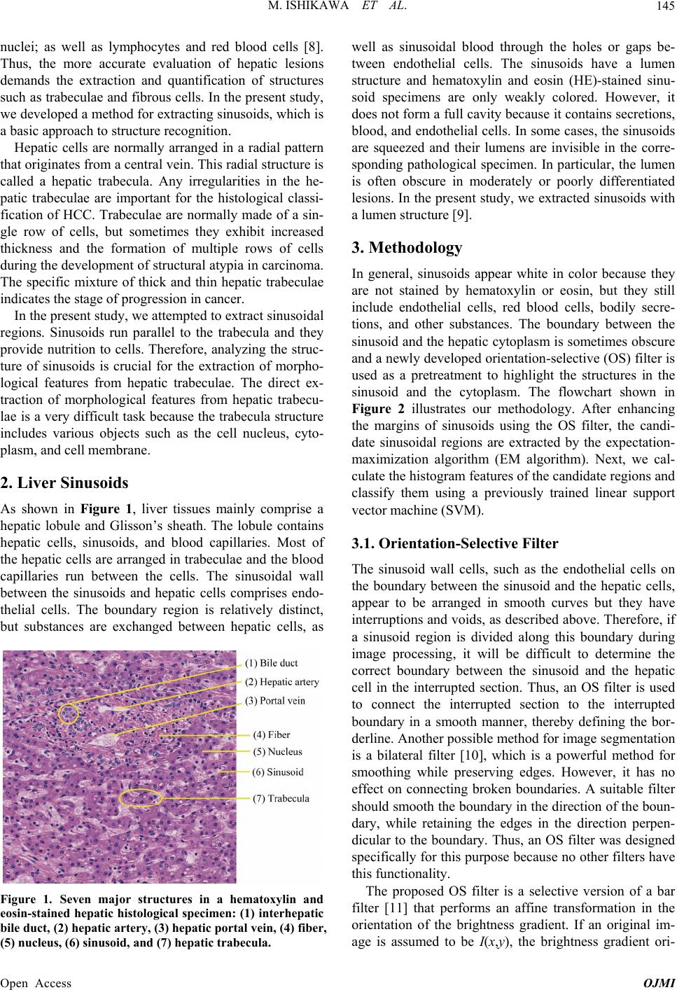 M. ISHIKAWA ET AL. 145 nuclei; as well as lymphocytes and red blood cells [8]. Thus, the more accurate evaluation of hepatic lesions demands the extraction and quantification of structures such as trabeculae and fibrous cells. In the present study, we developed a method for extracting sinusoids, which is a basic approach to structure recognition. Hepatic cells are normally arranged in a radial pattern that originates from a central vein. This radial structure is called a hepatic trabecula. Any irregularities in the he- patic trabeculae are important for the histological classi- fication of HCC. Trabeculae are normally made of a sin- gle row of cells, but sometimes they exhibit increased thickness and the formation of multiple rows of cells during the development of structural atypia in carcinoma. The specific mixture of thick and thin hepatic trabeculae indicates the stage of progression in cancer. In the present study, we attempted to extract sinusoidal regions. Sinusoids run parallel to the trabecula and they provide nutrition to cells. Therefore, analyzing the struc- ture of sinusoids is crucial for the extraction of morpho- logical features from hepatic trabeculae. The direct ex- traction of morphological features from hepatic trabecu- lae is a very difficult task because the trabecula structure includes various objects such as the cell nucleus, cyto- plasm, and cell membrane. 2. Liver Sinusoids As shown in Figure 1, liver tissues mainly comprise a hepatic lobule and Glisson’s sheath. The lobule contains hepatic cells, sinusoids, and blood capillaries. Most of the hepatic cells are arranged in trabeculae and the blood capillaries run between the cells. The sinusoidal wall between the sinusoids and hepatic cells comprises endo- thelial cells. The boundary region is relatively distinct, but substances are exchanged between hepatic cells, as Figure 1. Seven major structures in a hematoxylin and eosin-stained hepatic histological specimen: (1) interhepatic bile duct, (2) hepatic artery, (3) hepatic portal vein, (4) fiber, (5) nucleus, (6) sinusoid, and (7) hepatic trabecula. well as sinusoidal blood through the holes or gaps be- tween endothelial cells. The sinusoids have a lumen structure and hematoxylin and eosin (HE)-stained sinu- soid specimens are only weakly colored. However, it does not form a full cavity because it contains secretions, blood, and endothelial cells. In some cases, the sinusoids are squeezed and their lumens are invisible in the corre- sponding pathological specimen. In particular, the lumen is often obscure in moderately or poorly differentiated lesions. In the present study, we extracted sinusoids with a lumen structure [9]. 3. Methodology In general, sinusoids appear white in color because they are not stained by hematoxylin or eosin, but they still include endothelial cells, red blood cells, bodily secre- tions, and other substances. The boundary between the sinusoid and the hepatic cytoplasm is sometimes obscure and a newly developed orientation-selective (OS) filter is used as a pretreatment to highlight the structures in the sinusoid and the cytoplasm. The flowchart shown in Figure 2 illustrates our methodology. After enhancing the margins of sinusoids using the OS filter, the candi- date sinusoidal regions are extracted by the expectation- maximization algorithm (EM algorithm). Next, we cal- culate the histogram features of the candidate regions and classify them using a previously trained linear support vector machine (SVM). 3.1. Orientation-Selective Filter The sinusoid wall cells, such as the endothelial cells on the boundary between the sinusoid and the hepatic cells, appear to be arranged in smooth curves but they have interruptions and voids, as described above. Therefore, if a sinusoid region is divided along this boundary during image processing, it will be difficult to determine the correct boundary between the sinusoid and the hepatic cell in the interrupted section. Thus, an OS filter is used to connect the interrupted section to the interrupted boundary in a smooth manner, thereby defining the bor- derline. Another possible method for image segmentation is a bilateral filter [10], which is a powerful method for smoothing while preserving edges. However, it has no effect on connecting broken boundaries. A suitable filter should smooth the boundary in the direction of the boun- dary, while retaining the edges in the direction perpen- dicular to the boundary. Thus, an OS filter was designed specifically for this purpose because no other filters have this functionality. The proposed OS filter is a selective version of a bar filter [11] that performs an affine transformation in the orientation of the brightness gradient. If an original im- age is assumed to be I(x,y), the brightness gradient ori- Open Access OJMI  M. ISHIKAWA ET AL. Open Access OJMI 146 Figure 2. Flowchart of the proposed method: Section 3.1 is the pre-processing stage, Section 4.1 is the cluster ing process, and Section 4.4 is the discarding process. entation of each pixel is determined using Equation (1): 11 cossin 0 ,,sincos0 001 NS NS g ij , cijbijh ij 1, ,tan , yxy xy xxy (1) 1214, 8 ,0other xy bxy 22 ,1, ,,1, ,, 1, 1 , xxyIxy Ixy fyxyI xyI xy mxyfxxy fyxy (2) 22 2 1 ,exp 2π2 g2 y hxy (3) In the present study, a filter was used with Gaussian smoothing of 11 × 1 lines, where NS is the image size. The length of the filter is determined by the actual gaps being connected. In the present study, the filter was de- signed so it was two pixels shorter on either side com- pared to the size used to calculate the intensity gradient. If the filter is too large, intensity information other than that related to the sinusoid boundary would be included in the calculation. If there are two or more gradient ori- entations, these gradient orientations are calculated and integrated. The convolution-like operation in Equation (3) is performed using all of the RGB color channels. where θ(x,y) is the gradient orientation and m(x,y) is the gradient magnitude. The pixel values in the green chan- nel of the RGB color space are used because the differ- ence between the sinusoids and cytoplasm is relatively high [12]. Computing the orientation of a single pixel using only its four-connected neighborhood might be unstable, so we compute the pixel-wise orientation val- ues in three steps. First, we calculate the gradient of each pixel using centered 1D point derivatives with [−1, 0, +1] masks. Next, we quantize the gradient magnitudes into 18 equally spaced values between 0 and 170. Finally, we calculate the weighted gradient orientation histogram around each pixel in a neighborhood of 15 × 15 pixels. The size of the window is determined by the size of the object for which the intensity gradient is obtained. In the present study, this was slightly larger than the thickness of the sinusoid. The weights are the gradient magnitudes. The largest value in the weighted histogram is assigned to the center pixel. If multiple peaks in the histogram exceed 80% of the maximum, they are all assumed to be valid. This protects the structures of the edge crossings. This threshold is a parameter and when it is high, it gives greater priority to local edge enhancement, but more protection to edge crossings when it is low. Next, a bar filter is affine-transformed in the gradient orientation of each pixel and applied using Equation (3). This filter is similar to convolution, but the kernel depends on the weighted gradient orientation (θ) histogram described above. 3.2. Effectiveness of the Orientation-Selective Filter The filter used in the present study changes its convolu- tion kernel using spatial information, so the effects are also regarded as varying with the image properties. Thus, we examined whether the filter properties were suitable for sinusoid extraction from the hepatic histopathological tissue images considered in this study. First, the results of filtering are shown in Figure 3. Figures 3(a) and (b) show the original image and the results obtained by con- volution with the OS filter, respectively. Figure 4(b) shows the variation in a sinusoid where the gray level was obscure or a segment where favorable results were obtained compared with the original image (Figure 4(a)). Figure 4(c) shows the results obtained with the bilateral filter compared with the OS filter, where the cytoplasm around the sinusoid is clear, although the boundary be- tween the sinusoid and the cytoplasm is obscure. In the ,, l , ijIij Fcij  M. ISHIKAWA ET AL. 147 (a) (b) Figure 3. Original and filtered images. (a) Original image; (b) Orientation-selective filtered image. (a) (b) (c) Figure 4. Original and filtered images. (a) Original; (b) Ori- entation-selective filtered image; (c) Bilateral filtered image. results obtained after the application of the OS filter (Figure 4(b)), the boundary with the clear cytoplasm exhibits deeper pink eosin staining compared with the surrounding cytoplasm while the boundary between the sinusoid and the hepatic cell is more distinct because the sinusoid’s interior secretion is whiter as a consequence of smoothing. In addition, information related to the varia- tions in concentration from the sinusoid to the cytoplasm is conserved. 4. Extraction of Candidate Sinusoidal Regions HE-stained specimens mainly contain cell nuclei that appear blue due to hematoxylin, cytoplasm that appears red due to eosin, and sinusoids that appear white due to a lack of chemical reaction. We assumed that the signal intensities of the nuclei, cytoplasm, and sinusoids had Gaussian distributions in the RGB color space and we used the EM algorithm to estimate the corresponding class means and variances [13]. 4.1. Clustering with the EM Algorithm The EM algorithm is a well-established method that is often used often to estimate the parameters for mixed distribution models. In the present study, a mixed normal distribution was applied in the RGB color space to esti- mate the white region. An RGB feature vector is defined as, where N is the number of pixels in the image. The Gaussian mixture distribution can be defined using Equa- tion (4): 1 ;,, F kkk kk k pwwp xx 1 0, 1 F kk k ww 12 2 1 ;, 1 2π 1 exp 2 kkk d k T kk k p xx xx (4) where k is the average, k is the covariance matrix, k is the distribution weight, and F is the number of classes. In this case, the maximum likelihood estimate is represented by Equation (5). w 1 log ,logmax NF kk ik pwp xx 31 33 1 ,, ;,0, ,0,1 T kkk kkk F kkk k w ww (5) Open Access OJMI 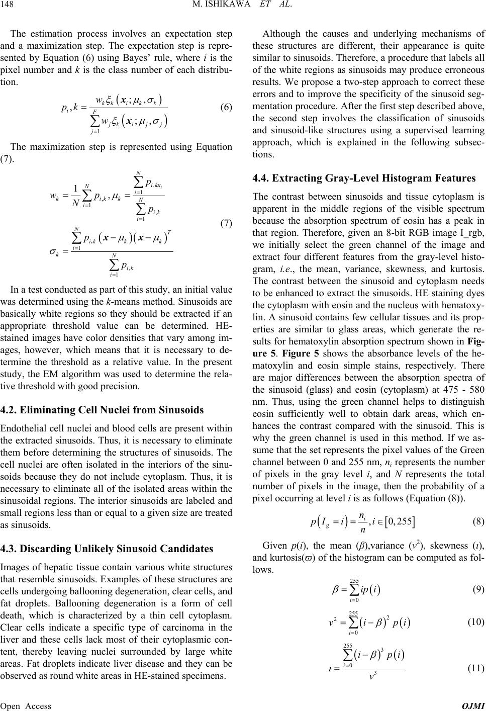 M. ISHIKAWA ET AL. 148 The estimation process involves an expectation step and a maximization step. The expectation step is repre- sented by Equation (6) using Bayes’ rule, where i is the pixel number and k is the class number of each distribu- tion. 1 ;, , ;, kki kk iF kijj j w pk w x x (6) The maximization step is represented using Equation (7). , 1 , 1 , 1 , 1 , 1 1, i N ik N i kikk N i ik i NT ik kk i kN ik i p wp Np p p x xx (7) In a test conducted as part of this study, an initial value was determined using the k-means method. Sinusoids are basically white regions so they should be extracted if an appropriate threshold value can be determined. HE- stained images have color densities that vary among im- ages, however, which means that it is necessary to de- termine the threshold as a relative value. In the present study, the EM algorithm was used to determine the rela- tive threshold with good precision. 4.2. Eliminating Cell Nuclei from Sinusoids Endothelial cell nuclei and blood cells are present within the extracted sinusoids. Thus, it is necessary to eliminate them before determining the structures of sinusoids. The cell nuclei are often isolated in the interiors of the sinu- soids because they do not include cytoplasm. Thus, it is necessary to eliminate all of the isolated areas within the sinusoidal regions. The interior sinusoids are labeled and small regions less than or equal to a given size are treated as sinusoids. 4.3. Discarding Unlikely Sinusoid Candidates Images of hepatic tissue contain various white structures that resemble sinusoids. Examples of these structures are cells undergoing ballooning degeneration, clear cells, and fat droplets. Ballooning degeneration is a form of cell death, which is characterized by a thin cell cytoplasm. Clear cells indicate a specific type of carcinoma in the liver and these cells lack most of their cytoplasmic con- tent, thereby leaving nuclei surrounded by large white areas. Fat droplets indicate liver disease and they can be observed as round white areas in HE-stained specimens. Although the causes and underlying mechanisms of these structures are different, their appearance is quite similar to sinusoids. Therefore, a procedure that labels all of the white regions as sinusoids may produce erroneous results. We propose a two-step approach to correct these errors and to improve the specificity of the sinusoid seg- mentation procedure. After the first step described above, the second step involves the classification of sinusoids and sinusoid-like structures using a supervised learning approach, which is explained in the following subsec- tions. 4.4. Extracting Gray-Level Histogram Features The contrast between sinusoids and tissue cytoplasm is apparent in the middle regions of the visible spectrum because the absorption spectrum of eosin has a peak in that region. Therefore, given an 8-bit RGB image I_rgb, we initially select the green channel of the image and extract four different features from the gray-level histo- gram, i.e., the mean, variance, skewness, and kurtosis. The contrast between the sinusoid and cytoplasm needs to be enhanced to extract the sinusoids. HE staining dyes the cytoplasm with eosin and the nucleus with hematoxy- lin. A sinusoid contains few cellular tissues and its prop- erties are similar to glass areas, which generate the re- sults for hematoxylin absorption spectrum shown in Fig- ure 5. Figure 5 shows the absorbance levels of the he- matoxylin and eosin simple stains, respectively. There are major differences between the absorption spectra of the sinusoid (glass) and eosin (cytoplasm) at 475 - 580 nm. Thus, using the green channel helps to distinguish eosin sufficiently well to obtain dark areas, which en- hances the contrast compared with the sinusoid. This is why the green channel is used in this method. If we as- sume that the set represents the pixel values of the Green channel between 0 and 255 nm, ni represents the number of pixels in the gray level i, and N represents the total number of pixels in the image, then the probability of a pixel occurring at level i is as follows (Equation (8)). ,0,255 i g n pI ii n i (8) Given p(i), the mean (β),variance (v2), skewness (ι), and kurtosis(ϖ) of the histogram can be computed as fol- lows. 255 0i ip i (9) 255 2 2 0i vip (10) 2553 0 3 i ip v i (11) Open Access OJMI 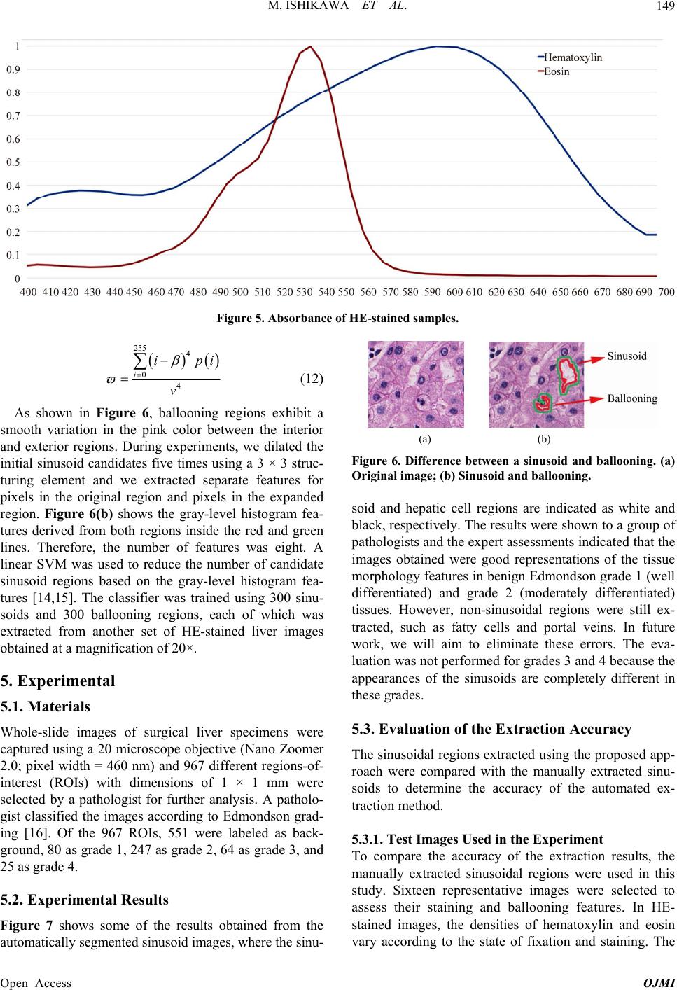 M. ISHIKAWA ET AL. Open Access OJMI 149 Figure 5. Absorbance of HE-stained samples. 255 4 0 4 i ip v i (12) As shown in Figure 6, ballooning regions exhibit a smooth variation in the pink color between the interior and exterior regions. During experiments, we dilated the initial sinusoid candidates five times using a 3 × 3 struc- turing element and we extracted separate features for pixels in the original region and pixels in the expanded region. Figure 6(b) shows the gray-level histogram fea- tures derived from both regions inside the red and green lines. Therefore, the number of features was eight. A linear SVM was used to reduce the number of candidate sinusoid regions based on the gray-level histogram fea- tures [14,15]. The classifier was trained using 300 sinu- soids and 300 ballooning regions, each of which was extracted from another set of HE-stained liver images obtained at a magnification of 20×. (a) (b) Figure 6. Difference between a sinusoid and ballooning. (a) Original image; (b) Sinusoid and ballooning. soid and hepatic cell regions are indicated as white and black, respectively. The results were shown to a group of pathologists and the expert assessments indicated that the images obtained were good representations of the tissue morphology features in benign Edmondson grade 1 (well differentiated) and grade 2 (moderately differentiated) tissues. However, non-sinusoidal regions were still ex- tracted, such as fatty cells and portal veins. In future work, we will aim to eliminate these errors. The eva- luation was not performed for grades 3 and 4 because the appearances of the sinusoids are completely different in these grades. 5. Experimental 5.1. Materials 5.3. Evaluation of the Extraction Accuracy Whole-slide images of surgical liver specimens were captured using a 20 microscope objective (Nano Zoomer 2.0; pixel width = 460 nm) and 967 different regions-of- interest (ROIs) with dimensions of 1 × 1 mm were selected by a pathologist for further analysis. A patholo- gist classified the images according to Edmondson grad- ing [16]. Of the 967 ROIs, 551 were labeled as back- ground, 80 as grade 1, 247 as grade 2, 64 as grade 3, and 25 as grade 4. The sinusoidal regions extracted using the proposed app- roach were compared with the manually extracted sinu- soids to determine the accuracy of the automated ex- traction method. 5.3.1. Test Images Used in the Experiment To compare the accuracy of the extraction results, the manually extracted sinusoidal regions were used in this study. Sixteen representative images were selected to assess their staining and ballooning features. In HE- stained images, the densities of hematoxylin and eosin vary according to the state of fixation and staining. The 5.2. Experimental Results Figure 7 shows some of the results obtained from the automatically segmented sinusoid images, where the sinu- 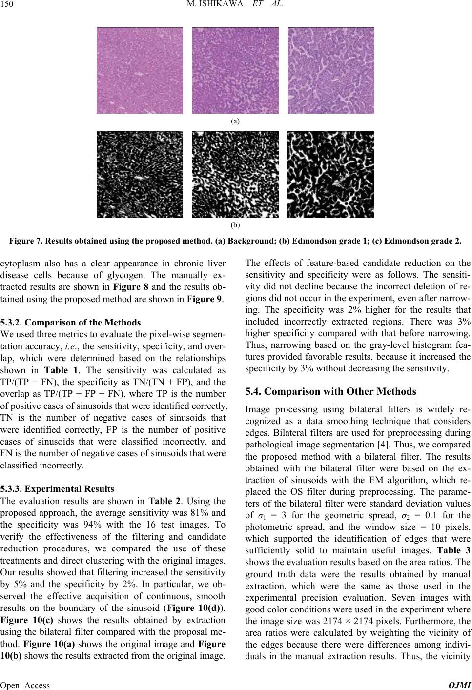 M. ISHIKAWA ET AL. 150 (a) (b) Figure 7. Results obtained using the propose d method. (a) Background; (b) Edmondson grade 1; (c) Edmondson gr ade 2. cytoplasm also has a clear appearance in chronic liver disease cells because of glycogen. The manually ex- tracted results are shown in Figure 8 and the results ob- tained using the proposed method are shown in Figure 9. 5.3.2. C omparison of the Metho d s We used three metrics to evaluate the pixel-wise segmen- tation accuracy, i.e., the sensitivity, specificity, and over- lap, which were determined based on the relationships shown in Table 1. The sensitivity was calculated as TP/(TP + FN), the specificity as TN/(TN + FP), and the overlap as TP/(TP + FP + FN), where TP is the number of positive cases of sinusoids that were identified correctly, TN is the number of negative cases of sinusoids that were identified correctly, FP is the number of positive cases of sinusoids that were classified incorrectly, and FN is the number of negative cases of sinusoids that were classified incorrectly. 5.3.3. Experimental Results The evaluation results are shown in Table 2. Using the proposed approach, the average sensitivity was 81% and the specificity was 94% with the 16 test images. To verify the effectiveness of the filtering and candidate reduction procedures, we compared the use of these treatments and direct clustering with the original images. Our results showed that filtering increased the sensitivity by 5% and the specificity by 2%. In particular, we ob- served the effective acquisition of continuous, smooth results on the boundary of the sinusoid (Figure 10(d)). Figure 10(c) shows the results obtained by extraction using the bilateral filter compared with the proposal me- thod. Figure 10(a) shows the original image and Figure 10(b) shows the results extracted from the original image. The effects of feature-based candidate reduction on the sensitivity and specificity were as follows. The sensiti- vity did not decline because the incorrect deletion of re- gions did not occur in the experiment, even after narrow- ing. The specificity was 2% higher for the results that included incorrectly extracted regions. There was 3% higher specificity compared with that before narrowing. Thus, narrowing based on the gray-level histogram fea- tures provided favorable results, because it increased the specificity by 3% without decreasing the sensitivity. 5.4. Comparison with Other Methods Image processing using bilateral filters is widely re- cognized as a data smoothing technique that considers edges. Bilateral filters are used for preprocessing during pathological image segmentation [4]. Thus, we compared the proposed method with a bilateral filter. The results obtained with the bilateral filter were based on the ex- traction of sinusoids with the EM algorithm, which re- placed the OS filter during preprocessing. The parame- ters of the bilateral filter were standard deviation values of σ1 = 3 for the geometric spread, σ2 = 0.1 for the photometric spread, and the window size = 10 pixels, which supported the identification of edges that were sufficiently solid to maintain useful images. Table 3 shows the evaluation results based on the area ratios. The ground truth data were the results obtained by manual extraction, which were the same as those used in the experimental precision evaluation. Seven images with good color conditions were used in the experiment where the image size was 2174 × 2174 pixels. Furthermore, the area ratios were calculated by weighting the vicinity of the edges because there were differences among indivi- duals in the manual extraction results. Thus, the vicinity Open Access OJMI 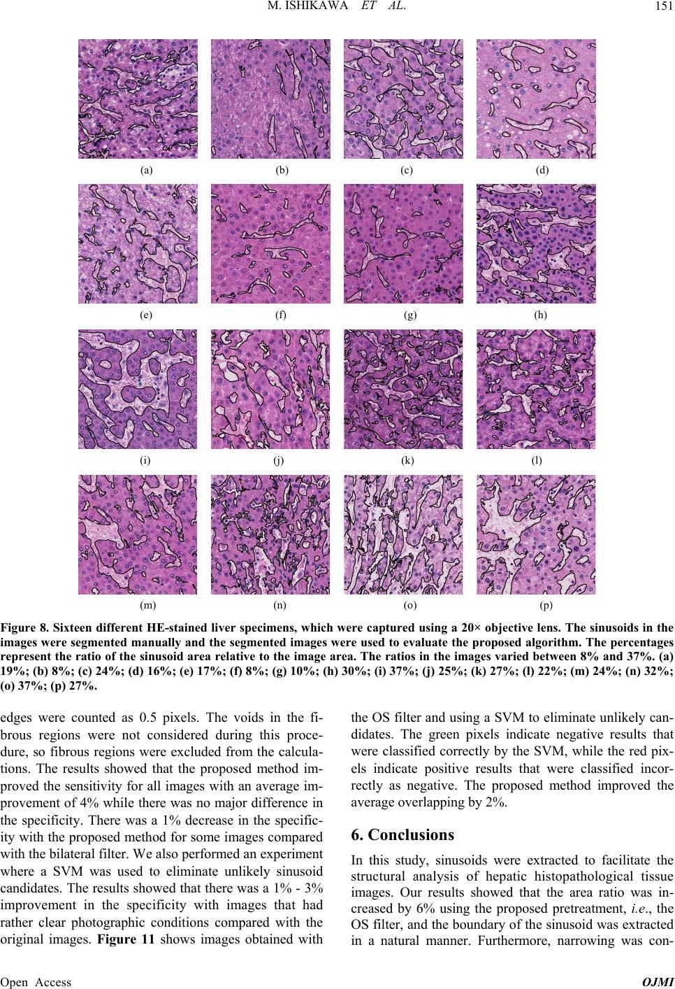 M. ISHIKAWA ET AL. 151 (a) (b) (c) (d) (e) (f) (g) (h) (i) (j) (k) (l) (m) (n) (o) (p) Figure 8. Sixteen different HE-stained liver specimens, which were captured using a 20× objective lens. The sinusoids in the images were segmented manually and the segmented images were used to evaluate the proposed algorithm. The percentages represent the ratio of the sinusoid area relative to the image area. The ratios in the images varied between 8% and 37%. (a) 19%; (b) 8%; (c) 24%; (d) 16%; (e) 17%; (f) 8%; (g) 10%; (h) 30%; (i) 37%; (j) 25%; (k) 27%; (l) 22%; (m) 24%; (n) 32%; (o) 37%; (p) 27%. edges were counted as 0.5 pixels. The voids in the fi- brous regions were not considered during this proce- dure, so fibrous regions were excluded from the calcula- tions. The results showed that the proposed method im- proved the sensitivity for all images with an average im- provement of 4% while there was no major difference in the specificity. There was a 1% decrease in the specific- ity with the proposed method for some images compared with the bilateral filter. We also performed an experiment where a SVM was used to eliminate unlikely sinusoid candidates. The results showed that there was a 1% - 3% improvement in the specificity with images that had rather clear photographic conditions compared with the the OS filter and using a SVM to eliminate unlikely can- didates. The green pixels indicate negative results that were classified correctly by the SVM, while the red pix- els indicate positive results that were classified incor- rectly as negative. The proposed method improved the average overlapping by 2%. 6. Conclusions original images. Figure 11 shows images obtained with oids were extracted to facilitate the In this study, sinus structural analysis of hepatic histopathological tissue images. Our results showed that the area ratio was in- creased by 6% using the proposed pretreatment, i.e., the OS filter, and the boundary of the sinusoid was extracted in a natural manner. Furthermore, narrowing was con- Open Access OJMI 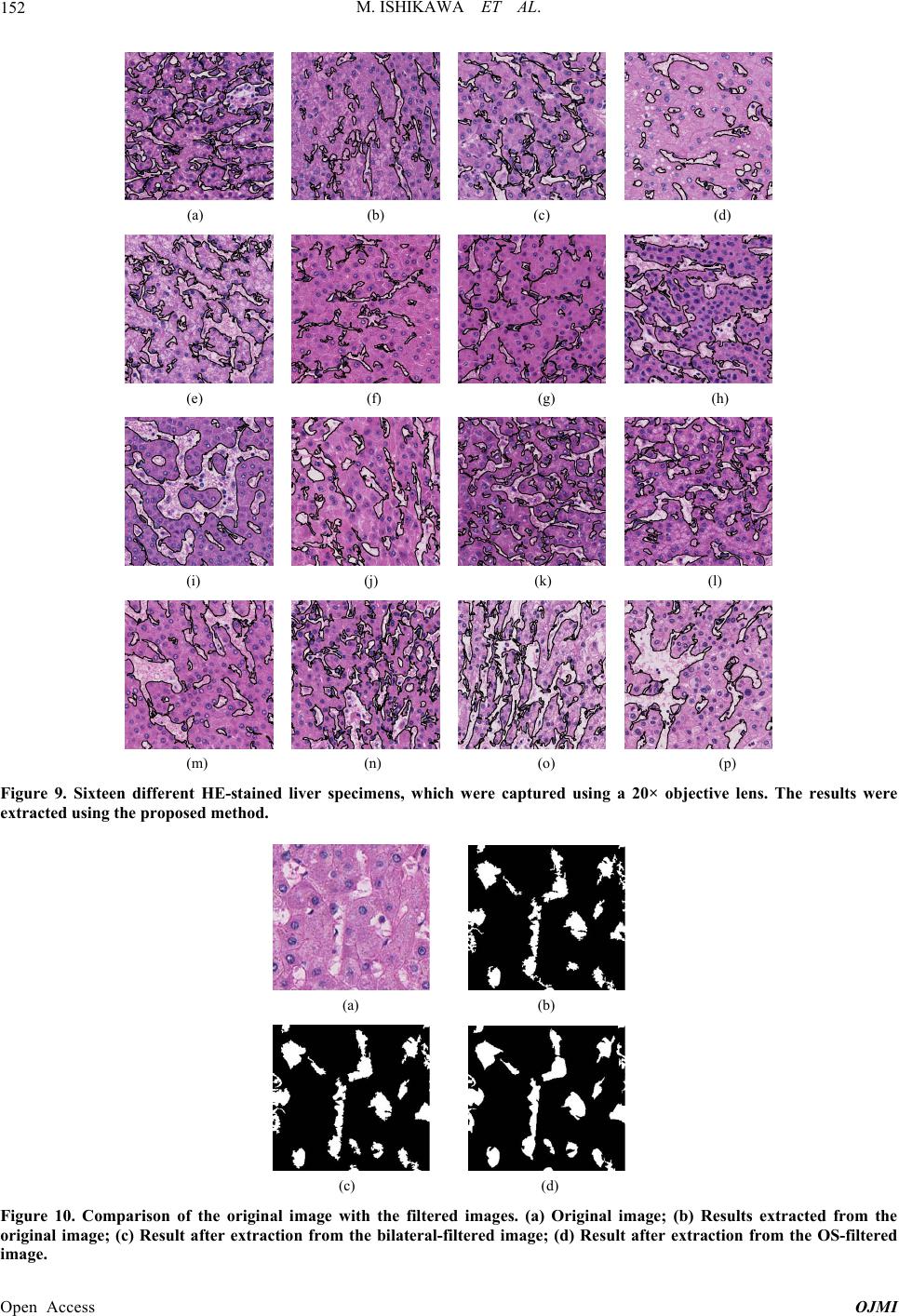 M. ISHIKAWA ET AL. 152 (a) (b) (c) (d) (e) (f) (g) (h) (i) (j) (k) (l) (m) (n) (o) (p) Figure 9. Sixteen differens.he results were extracted using the propo t HE-stainever specimens, where captured usin20× objective len sed method. d liich wg a T (a) (b) (c) (d) Figure 10. Comparison of the original image iginal image; (b) Results extracted from the original image; (c) Result after extraction from) Result after extraction from the OS-filtered image. with the filtages. (a) Or the bilateral-filtered image; (d ered im Open Access OJMI 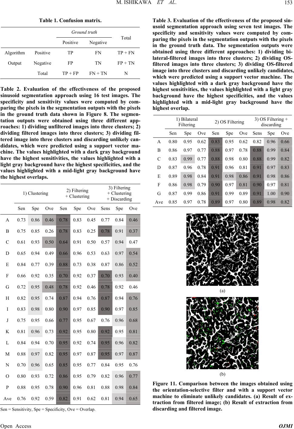 M. ISHIKAWA ET AL. 153 Table 1. Confusion matrix. Ground truth e Total Positive Negativ Algorithm Positive T TP + FN P FN Output Negative FP TPP FN FP TN + TN Total + F + TNN Tavaf theenef thed sinusoid segmentation apsin imagThe ecificity and sensitivity values were computed by com- + Discarding ble 2. Eluation o effectivss o propose proach ug 16 testes. sp paring the pixels in the segmentation outputs with the pixels in the ground truth data shown in Figure 8. The segmen- tation outputs were obtained using three different app- roaches: 1) dividing unfiltered images into three clusters; 2) dividing filtered images into three clusters; 3) dividing fil- tered image into three clusters and discarding unlikely can- didates, which were predicted using a support vector ma- chine. The values highlighted with a dark gray background have the highest sensitivities, the values highlighted with a light gray background have the highest speci ficities, and the values highlighted with a mid-light gray background have the highest overlaps. 1) Clustering 2) Filtering + Clustering 3) Filtering + Clustering Sen Spe Ove Sen Spe SenveOve s SpeO A 0.73 0.86 0.46 0.778 0.83 0.45 0.7 0.84 0.46 B 0.75 0.85 0.26 0.78 0.83 0.25 0.78 0.910.37 C 0.61 0.93 0.50 0.64 0.91 0.50 0.57 0.94 0.47 D 0.65 0.94 0.49 0.66 0.96 0.53 0.63 0.97 0.54 E 0.84 0.77 0.39 0.88 0.73 0.38 0.87 0.86 0.52 F 0.66 0.92 0.35 0.70 0.92 0.37 0.70 0.930.40 G 0.72 0.95 0.48 0.78 0.92 0.46 0.78 0.92 0.46 H 0.82 0.95 0.74 0.87 0.94 0.76 0.87 0.94 0.76 I 0.83 0.98 0.80 0.90 0.97 0.85 0.90 0.97 0.85 J 0.75 0.95 0.66 0.77 0.95 0.67 0.76 0.96 0.68 K 0.81 0.96 0.73 0.92 0.95 0.80 0.92 0.95 0.81 L 0.84 0.94 0.70 0.95 0.92 0.74 0.95 0.960.82 M 0.88 0.97 0.82 0.95 0.97 0.87 0.95 0.970.87 N 0.70 0.96 0.65 0.85 0.95 0.77 0.84 0.95 0.76 O 0.80 0.93 0.72 0.86 0.95 0.79 0.82 0.96 0.77 P 0.88 0.95 0.78 0.90 0.96 0.81 0.88 0.98 0.84 A ve 0.76 0.92 0.59 0.82 0.91 0.62 0.81 0.94 0.65 Sen = Sensitivity, Spe = Specificity, Ove = Overlap. specificity and sensitivity values were computed by com- paring the pixels in the segmentation outputs with the pixels in the gr ntationere ob ineddifferches: 1) dividing bi- lateral-filtered images into three clusters; 2)S- filteredgteus il image into three clusters and discarding unlikely candidates, wh cs e values highlighted k hsie valuesl t s, and the values Table 3. Evaluation of the effectiveness of the proposed sin- usoid segmentation approach using seven test images. The ound truth data. using three The segme outputs w taent approa dividing O imaes ino thre clters;3) dividing OS-ftered hicwerepredited uing asupport vector machin. The with a dark gr s, theay high bac ighted ground have with the grayighet senstivitia ligh background have the highest specificitie highlighted with a mid-light gray background have the highest overlap. 1) Bilateral Filtering 2) OS Filtering 3) OS Filtering + discarding SenSpeOveSenSpe Ove Sens SpeOve A0.800.95 0.620.83 0.95 0.62 0.82 0.960.66 B0.860.97 0.77 0.88 0.97 0.78 0.88 0.990.84 C0.83 0.99 0.770.88 0.98 0.80 0.88 0.990.82 D0.870.96 0.780.91 0.96 0.81 0.91 0.970.83 E0.89 0.980.840.910.98 0.86 0.91 0.980.86 F0.86 0.980.790.900.97 0.81 0.90 0.97 0.81 G0.870.99 0.860.91 0.99 0.89 0.91 1.000.90 Ave0.88 0. 50.97 0.789 0.97 0.80 0.89 0.980.82 (a) (b) Figure 11. Comparison between the images obtained using the orientation-selective filter and with a support vector machine to eliminate unlikely candidates. (a) Result of ex- traction from filtered image; (b) Result of extraction from discarding and filtered image. Open Access OJMI 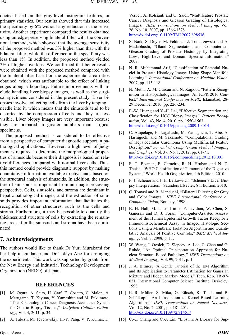 M. ISHIKAWA ET AL. 154 ducted based on the gray-level histogram features, or primary statistics. Our results showed that this increased the specificity by 6% without any reduction in the sensi- tivity. Another experiment compared the results obtained using an edge-preserving bilateral filter with the conven- tional method, which showed that the average sensitivity of the proposed method was 3% higher than that with the bilateral filter, while the difference in the specificity was less than 1%. In addition, the proposed method yielded 2% of higher overlaps. We confirmed that better results were obtained with the proposed method cmpared with the bilateral filter based one experimental area ratios Tabesh, M. Teverovskiy, H.-Y. Pang, V. P. Kumar, D. . Saidi, “Multifeature Prostate o th obtained, which was attributable to the effect of linking edges along a boundary. Future improvements will in- clude handling liver biopsy images, as well as the surgi- cal specimens considered in the present study. Liver bi- opsies involve collecting cells from the liver by tapping a needle into it, which means that the sinusoids tend to be distorted by the compression of cells and they are less visible. Liver biopsy images are very important because they are prepared in greater numbers than surgical specimens. The proposed method is considered to be effective from a perspective of computer diagnostic support in pa- thological applications. However, a high level of judg- ment is required to determine the morphological proper- ties of sinusoids because their diagnosis is based on rela- tive differences compared with normal liver cells. Thus, this method could provide diagnostic support by making quantitative information available to physicians based on the structural analysis of sinusoids. In addition, the struc- ture of sinusoids is important from an image processing perspective. Cells, sinusoids, and stroma are dominant in hepatic pathological images, and the extraction of sinu- soids provides important information that facilitates the recognition of other structures, such as the cells and stroma. Furthermore, it may be possible to quantify the thickness and structure of cells by extracting the remain- ing areas after the sinusoids and stroma have been elimi- nated. 7. Acknowledgements The authors would like to thank Dr Yuri Murakami for her helpful guidance and Dr Tokiya Abe for arranging the experiments. This work was supported by grants from the New Energy and Industrial Technology Development Organization (NEDO) of Japan. REFERENCES [1] M. Ogura, A. Saito, H. Graf, E. Cosatto, C. Malon, A. Marugame, T. Kiyuna, Y. Yamashita and M. Fukumoto, “The E-Pathologist Cancer Diagnosis Assistance System for Gastric Biopsy Tissues,” Analytical Cellular Pathol- ogy, Vol. 4, 2011, p. 34. [2] A. Verbel, A. Kotsianti and O Cancer Diagnosis and Gleason Grading of Histological Images,” IEEE Transactions on Medical Imaging, Vol. 26, No. 10, 2007, pp. 1366-1378. http://dx.doi.org/10.1109/TMI.2007.898536 [3] S. Naik, S. Doyle, M. Feldman, J. Tomaszewski and A. Madabhushi, “Gland Segmentation and Computerized Gleason Grading of Prostate Histology by Integrating Low-, High-Level andrmation,” 2007. N. Rajpoot, “Pattern Recog- Pattern Recog- Domain Specific Info [4] N. R. Muhammad Arif, “Classification of Potential Nu- clei in Prostate Histology Images Using Shape Manifold Learning,” International Conference on Machine Vision, 2007, pp. 113-118. [5] N. Metin, A. M. Gurcan and nition in Histopathological Images: An ICPR 2010 Con- test,” International Conference on ICPR, Islamabad, 28- 29 December 2010, pp. 226-234. [6] P.-W. Huang and Y.-H. Lai, “Effective Segmentation and Classification for HCC Biopsy Images,” nition, Vol. 43, No. 4, 2010, pp. 1550-1563. http://dx.doi.org/10.1016/j.patcog.2009.10.014 [7] C. Atupelage, H. Nagahashi, M. Yamaguchi, T. Abe, A. Hashiguchi and M. Sakamoto, “Computational Grading of Hepatocellular Carcinoma Using Multifractal Feature Description,” Journal of Computerized Medical Imaging and Graphics, Vol. 37, No. 1, 2012, pp. 61-71. http://dx.doi.org/10.1016/j.compmedimag.2012.10.001 [8] F. T. Bosman, F. Carneiro, R. H. Hruban and N. D. Theise, “WHO Classification of Tumours of the Digestive ateral Filtering for Gray Chen, S. d Assess- . System,” World Health Organization, 4th Edition, 2010. [9] P. J. Scheuer and J. H. Lefkowitch, “Scheuer’s Liver Bio- psy Interpretation,” Saunders Elsevier, 8th Edition, 2010. [10] C. Tomasi and R. Manduchi, “Bil and Color Images,” IEEE International Conference on Computer Vision, Bombay, 1998. [11] B. H. Hall, M. Ianosi-Irimie, P. Javidian, W. Ganesan and D. J. Foran, “Computer-Assiste ment of the Human Epidermal Growth Factor Receptor 2 Immunohistochemical Assay in Imaged Histologic Sec- tions Using a Membrane Isolation Algorithm and Quanti- tative Analysis of Positive Controls,” BMC Medical Im- aging, Vol. 8, 2008, p. 11. [12] W. Wang, J. Ozolek, D. Slepcev, A. Lee, C. Chen and G Rohde, “An Optimal Transportation Approach for Nu- clear Structure-Based Pathology,” IEEE Transactions on Medical Imaging, Vol. 99, 2011, p. 1. [13] J. A. Bilmes, “A Gentle Tutorial of the EM Algorithm and Its Application to Parameter Estimation for Gaussian Mixture and Hidden Markov Models,” Tech. Rep. TR-97- 021, International Computer Science Institute, Berkeley, 1998. [14] K.-R. Müller, S. Mika, G. Rätsch, K. Tsuda and B. Schölkopf, “An Introduction to Kernel-Based Learning Algorithms,” IEEE Transactions on Neural Networks, Vol. 12, No. 2, 2001, pp. 181-201. http://dx.doi.org/10.1109/72.914517 [15] C.-C. Chang and C.-J. Lin, “Libsvm: A Library for Sup- Open Access OJMI  M. ISHIKAWA ET AL. Open Access OJMI 155 M Transactions on Intelligentport Vector Machines,” AC Systems and Technology, Vol. 2, No. 3, 2011, pp. 1-7. http://dx.doi.org/10.1145/1961189.1961199 [16] H. A. Edmondson and P. E. Steiner, “Primary Carcinoma of the Liver: A Study of 100 Case cropsies,” Cancer, Vol. 7, No. 3, 1954 s among 48,900 Ne- , pp. 462-503. http://dx.doi.org/10.1002/1097-0142(195405)7:3<462::AI D-CNCR2820070308>3.0.CO;2-E
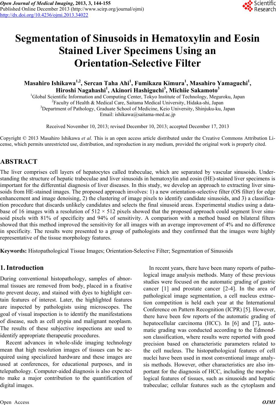
|