Engineering, 2013, 5, 413-415
http://dx.doi.org/10.4236/eng.2013.510B084 Published Online October 2013 (http://www.scirp.org/journal/eng)
Copyright © 2013 SciRes. ENG
Optimal Estimation of Parameters for an HIV Model
Danna Sun, Zhaoying Jiang, Ziku Wu*
College of Science and Information, Qingdao Agricultural University, Qingdao, China
Email: msj1958@126.com, *zkwu1968@126.com
Received 2013
ABSTRACT
An HIV model was considered. The parameters of the model are estimated by adjoint dada assimilation method. The
results showed the method is valid. This method has potential application to a wide variety of models in biomathemat-
ics.
Keywords: HIV Model; Optimal Estimation; Adjoint Data Assimilation
1. Introduction
One of the worst diseases in the world is AIDS (Ac-
quired Immunity Deficiency Syndrome). It is caused by
the human immunodeficiency virus (HIV). There has
been much interest recently in mathematical models of
HIV. During the last decade, many scholars have done a
great of work about HIV model ([1-6]). We consider a
model which presented by Henry et al. ([1]), which de-
scribes the interaction of HIV and the immune system of
the body. In this model, the variables are uninfected CD4
+ T-cells, infected such cells and free virus, whose densi-
ties at time t are denoted respectively by
()xt
,
()yt
and
()vt
. These quantity satisfy
0
0
0
dx s x xy
dt
dy xy y
dt
dv cy v
dt
µβ
βα
γ
−+ +=
− +=
−+ =
(1)
with initial values
(0) 0x>
,
(0) 0y
and
(0) 0v>
.
Here s,
µ
,
β
,
, c and
γ
are model parameters
which interpreted as follows:
s: is the rate of pro duc tion of CD4 + T-cells
: is their per capita death rate
: is the rate of infection of CD4 + T-cells by virus
: is the per capita rate of disappearance of infected
cells
c: is the rate of production of virus by infected cells
γ
: is the death rate of virus particles.
It’s impossible to get the above model’s analytic solu-
tions due to its strong nonlinearity. Thus we computed its
solutions using Runge-Kutta methods of order 4. This
was done with initial Thu s we computed its solutions us-
ing Runge-Kutta methods of order 4. This was done with
initial (0) 200
x
=,
(0) 0y=
and
(0) 1v=
, and typical
parameters values
0.272s=
,
0.00136
µ
=
, β =
0.00027,
0.33
α
=
,
50c=
and
2
γ
=
. The time series
of uninfected CD4+T-cells and infected CD4 + T-cells
are listed in Figures 1 and 2, res pectively. The peak val-
ues exist round 20 days. The phase portraits are shown in
Figure 3 for a time period of 200 d ays and it can be seen
that the orbits are quite close.
These model parameters are chosen to be consistent
with those in the model, whose values may not be very
well known. There has recently been considerable inter-
est in the inverse problem of determining such values by
incorporating measured data into the numerical model.
The adjoint assimilation method involves minimizing a
certain cost function which consists basically of a norm
of the difference between the computed and the observed
values of the measured variables. The purpose of the
Figure 1. The time series of uninfected CD4 + T-cell.
*Corresponding a uthor.
D. N. SUN ET AL.
Copyright © 2013 SciRes. ENG
414
Figure 2. The time series of infected CD4 + T-cell.
Figure 3. The phase portraits.
present paper is to estimate the model parameters (μ, α, λ)
by constructing the adjoint model. The basis of the me-
thod is to minimize the cost function which is equal to a
norm of difference between the computed and the ob-
served data. An algorithm is obtained, via so-called ad-
joint equation, for construction of the gradient of the
function with respect to the parameters.
In Section 2 we describe the adjoint assimilation me-
thod. A detailed discussion of the numerical tests results
is given in Section 3. Section 4 summarizes the results
and conclusions.
2. The Adjoint Numerical Model
For parameter estimation and data assimilation, differ-
ences between predicted and measured values of these
variables must be quantified by a single misfit number,
the objective function. A lot of options are available for
choosing the misfit function. In this study, we choose the
classical least-squares approach. However, the results
from above governing equations are not good as with the
observed values. The error between observed and model
calculated can be defined as
2 22
12 3
0
1(()()())
2
To oo
Jw xxwyywvvdt=−+ −+−
(2)
Where
o
x
,
o
y
and
o
v
present observation of x, y and
v, respectively.
1
w
,
2
w
and 3
w
are weight coeffi-
cients and
[0, ]T
stands for assimilation window.
In order to get the adjoint Equations of (1), we intro-
duce the adjoint control variables and Lagrange function:
0
()
T
LJXLxYLyVLv dt=+ ++
(3)
where X, Y and V are adjoint variables.
Lx
,
Ly
, and
Lv
are the left hand part of Equations (1). It is easy to
get the following adjoint equations:
1
2
3
()()0
( )0
() ()0
o
o
o
dX XvXYw xx
dt
dY YcVw yy
dt
dV VxXYw vv
dt
µβ
α
γβ
− ++−+− =
−+−+− =
−+ +−+−=
(4)
Now the parameters
,
α
and
γ
are unknown,
which need to estimate by the adjoint assimilation me-
thod. The numerical scheme of the adjoint Equation (4)
are the same as Equation (1), however it needs to inte-
grate backward, and its initial conditions are set to zeros,
that is
()0,()0,()0
Xt YTVT=== (5)
The gradients can be easily obtained through Equation
(3), which are
0
0
0
T
T
T
JxXdt
JyYdt
JvVdt
µ
α
γ
=
=
=
(6)
For the sake of convenience, we denotes
'
(,,)P
µαγ
=
(7)
(, ,)
JJJJ
P
µαγ
∂∂∂
∇=
∂∂∂
(8)
Having determined the gradients which respect to the
unknown parameters, we can perform the minimization
by the descend method, the modified parameters are
pa pagd
λ
⇐ −×
(9 )
where
λ
is the optimal step.
D. N. SUN ET AL.
Copyright © 2013 SciRes. ENG
415
3. Numerical Tests
In real applications, the model must be calibrated against
experimental data. In this numerical study, however, a
twin experiment is carried out: a reference solution is
generated with the model itself using the parameters the
same as in Section I.
In this part, we design 3 numerical tests, 2 tests with
random error in the synthetic data, which denoted TX1
with no errors, TX2 with 1% errors, TX3 with 3% errors,
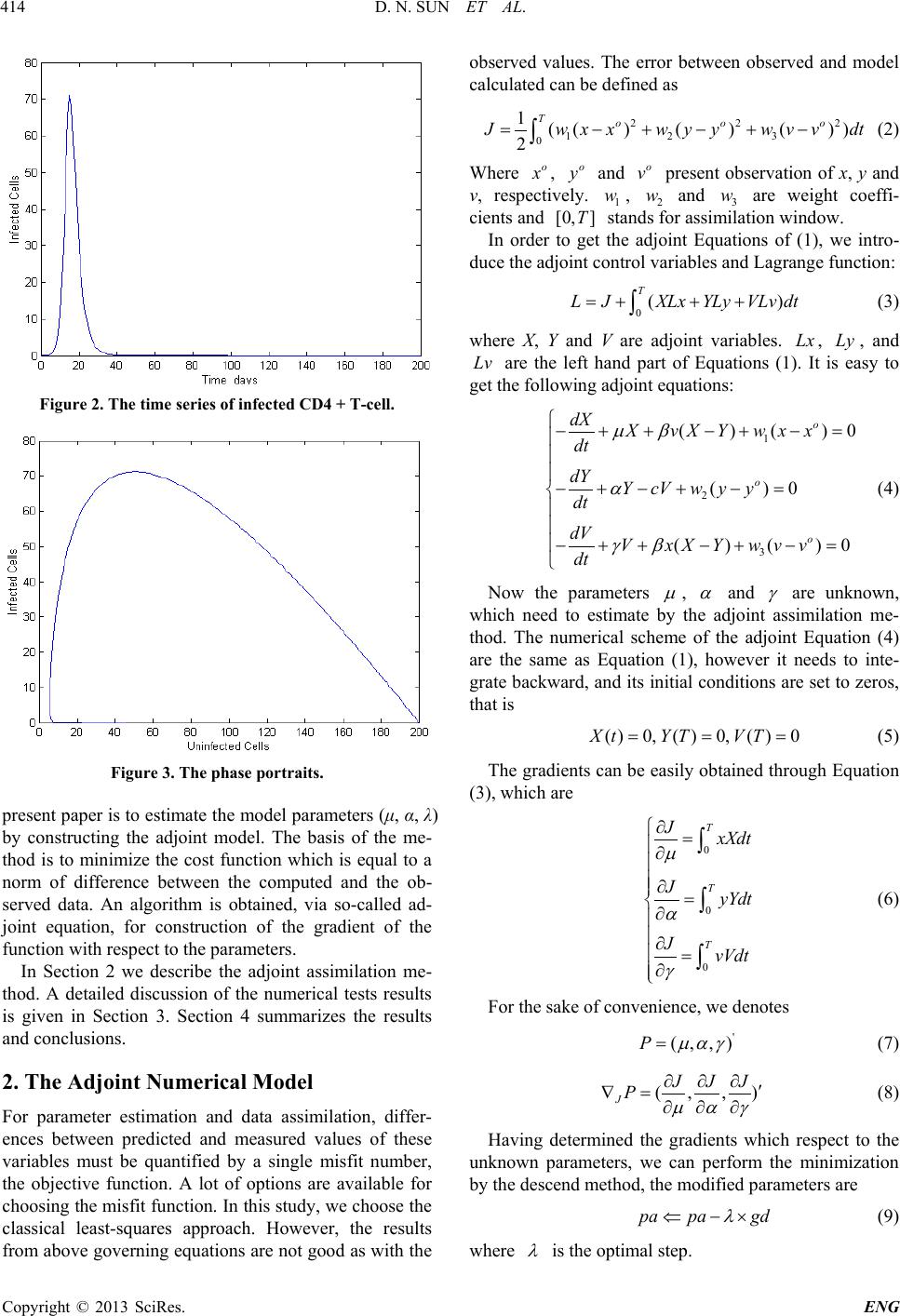
respectively. Only the infected CD4 + T-cells observed
data are valid, that is
13
0ww= =
. The first guess of
them are 1.0E3, 0.2 and 1.5, respectively. The observed
dada are plotted in Figure 4. Th e numerical resu lts listed
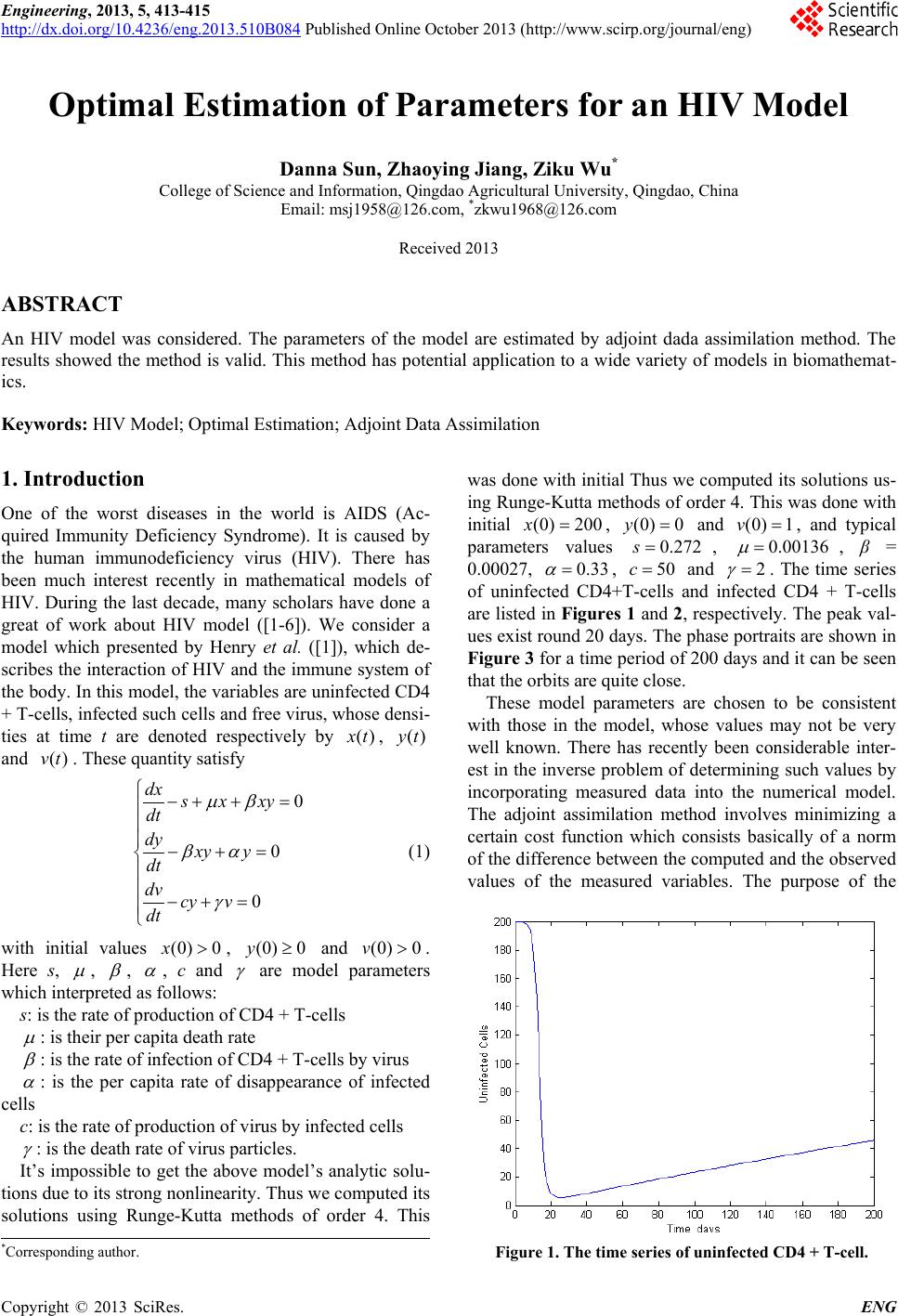
in Table 1. The cost function descent curve showed in
Figure 5.
4. Summary and Discussion
Adjoint data assimilation method is employed to estimate
the parameters of a kind of HIV model. The parameters
estimated are μ, α and γ. The method is based on an op-
timal control approach where by a cost function measur-
ing the discrepancies between numerical computed and
measured is minimized, subject to constrains consisting
of equations of the model. The numerical scheme used is
the forth order Runge-Kutta method. In order to test the
validity of this method, we have designed several expe-
riments. The results showed the method is valid. The
research results are useful to understand the HIV model
and helpful to establish a robust and effective HIV con-
trol and prediction.
Figure 4. The observed data.
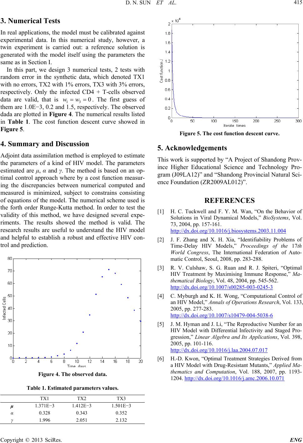
Table 1. Estimated parameters values.
TX1 TX2 TX3
μ 1.371E3 1.412E3 1.501E3
α 0.328 0.343 0.352
γ 1.996 2.051 2.132
Figure 5. The cost f unction desc ent curve.
5. Acknowledgements
This work is supported by “A Project of Shandong Prov-
ince Higher Educational Science and Technology Pro-
gram (J09LA12)” and “Shandong Provincial Natural Sci-
ence Foundation (ZR2009AL012)”.
REFERENCES
[1] H. C. Tuckwell and F. Y. M. Wan, “On the Behavior of
Solutions in Viral Dynamical Models,” BioSystems, Vol.
73, 2004, pp. 157-161.
http://dx.doi.org/10.1016/j.biosystems.2003.11.004
[2] J. F. Zhang and X. H. Xia, “Identifiability Problems of
Time-Delay HIV Models,” Proceedings of the 17th
World Congress, The International Federation of Auto-
matic Control, Seoul, 2008, pp. 283-288.
[3] R. V. Culshaw, S. G. Ruan and R. J. Spiteri, “Optimal
HIV Treatment by Maximising Immune Response,” Ma-
thematical Biology, Vol. 48, 2004, pp. 545-562.
http://dx.doi.org/10.1007/s00285-003-0245-3
[4] C. Myburgh and K. H. Wong, “Computational Control of
an HIV Model,” Annals of Operations Research, Vol. 133,
2005, pp. 277-283.
http://dx.doi.org/10.1007/s10479-004-5038-6
[5] J. M. Hy ma n and J. Li, “The Reproductive Number for an
HIV Model with Differential Infectivity and Staged Pro-
gression,” Linear Algebra and Its Applications, Vol. 398,
2005, pp. 101-116.
http://dx.doi.org/10.1016/j.laa.2004.07.017
[6] H.-D. Kwon, “Optimal Treatment Strategies Derived from
a HI V Model with Drug-Resistant Mutants,” Applie d Ma-
thematics and Computation, Vol. 188, 2007, pp. 1193-
1204. http://dx.doi.org/10.1016/j.amc.2006.10.071