 International Journal of Intelligence Science, 2014, 4, 7-16 Published Online January 2014 (http://www.scirp.org/journal/ijis) http://dx.doi.org/10.4236/ijis.2014.41002 OPEN ACCESS IJIS Soccer League Competition Algorithm, a New Method for Solving Systems of Nonlinear Equations Naser Moosavian, Babak Kasaee Roodsari Department of Civil Engineering, Ferdowsi University of Mashhad, Mashhad, Iran Email: naser.moosavian@yahoo.com Received October 9, 2013; revised November 9, 2013; accepted November 15, 2013 Copyright © 2014 Naser Moosavian, Babak Kasaee Roodsari. This is an open access article distributed under the Creative Commons Attribution License, which permits unrestricted use, distribution, and reproduction in any medium, provided the original work is properly cited. In accordance of the Creative Commons Attribution License all Copyrights © 2014 are reserved for SCIRP and the owner of the intellectual property Naser Moosavian, Babak Kasaee Roodsari. All Copyright © 2014 are guarded by law and by SCIRP as a guardian. ABSTRACT This paper introduces Soccer League Competition (SLC) algorithm as a new optimization technique for solving nonlinear systems of equations. Fundamental ideas of the method are inspired from soccer leagues and based on the competitions among teams and players. Like other meta-heuristic methods, the proposed technique starts with an initial population. Population individuals called players are in two types: fixed players and substitutes that all together form some teams. The competition among teams to take the possession of the top ranked posi- tions in the league table and the internal competitions between players in each team for personal improvements results in the convergence of population individuals to the global optimum. Results of applying the proposed al- gorithm in solving nonlinear systems of equations demonstrate that SLC converges to the answer more accu- rately and rapidly in comparison with other Meta-heuristic and Newton-type methods. KEYWORDS Soccer League Competition; Nonlinear Equations; Meta-Heuristic Algorithm 1. Introduction Solving systems of nonlinear equations is one of the main concerns in a diverse range of engineering applica- tions such as computational mechanics, weather forecast, hydraulic analysis of water distribution systems, aircraft control and petroleum geological prospecting. Many pre- vious efforts have been made to find a solution for sys- tems of nonlinear equations. Results of these studies comprise some theories and algorithms [1-4]. Among such approaches, Newton’s method is one of the most powerful numerical methods and an important basic me- thod which has a quadratic convergence if the function F is continuously differentiable and if a good initial guess x0 is provided [5]. Frontini and Sormani [6] proposed a third-order method based on a quadrature formula to solve systems of nonlinear equations. Cordero and Tor- regrosa [7] developed some variants of Newton’s method based on trapezoidal and midpoint rules of quadrature. Also, Darvishi and Barati [8-10] presented some high order iterative methods and Babajee et al. [11] proposed a fourth-order iterative technique. Luo et al. [12] solved a system of nonlinear equations using a combination of chaos search and Newton-type methods. More recently, Mo et al. [5] presented a combination of the conjugate direction method (CD) and particle swarm optimization (PSO) for solving systems of nonlinear equations. The convergence and performance characteristics of Newton-type methods are highly sensitive to the initial guess of the solution supplied to the methods and the algorithm would fail if the initial guess of the solution is improper. However, it is difficult to select a good initial guess for most systems of nonlinear equations [13]. The system of nonlinear equations is considered as follows: 112 212 12 ,,, 0 ,,, 0 ,,, 0. n n nn fxx x fxx x fxxx (1) Applying the global optimization methods, the system  N. MOOSAVIAN, B. K. ROODSARI 8 of Equation (1) is transformed to an optimization prob- lem. This is achieved by using the auxiliary function: 2 12 1 min,, ,, n i i n fxx xxx x (2) Global minimum of above formulation is zero and is a root for the corresponding system of equations if . This paper presents a new meta-heuristic algorithm, called Soccer League Competitions (SLC), for solving Equation (2). * x *0Fx In Section 2, the basic concepts of SLC are defined. In Section 3, the performance and effectiveness of SLC are validated by some examples. Finally, the conclusions are presented in Section 4. 2. Soccer League Competitions Level one soccer league consists of teams (clubs) com- peting each other during a season. In this environment, some stronger teams aim to sit in the first positions of the league table while some weaker teams plan to survive in the level one league in order to prevent a crash out to the second level league. During the course of a season, each team plays the others twice, once at their home stadium and once at that of their opponents. Teams receive 3 points for a win and no point is awarded for a lost. Teams are weekly ranked by total points and the club with the most point is crowned champion at the end of each sea- son. The number of matches in each season depends on the team numbers. For instance, in a league consisting of M teams the total number of matches is calculated as follows: Total Match12MM (3) In this league, each team participates in 1 inde- pendent matches, and totally, 12MM compe- titions are being held during a season. There is always an intense competition between the teams at the bottom of the league table. As a rule, the two bottom table teams are crashed out to the second level soccer league (relegations spots) at the end of the season. In return, two first table teams of the second level league (promotions spots) replaced with the relegated teams. Generally, promotions spots import new players to the league which may have potential of being a future star. Each team consists of 11 fixed players (FP) and some substitutes (S). A team’s power depends on the power of its players. Moreover, powerful teams have a higher chance of winning their matches. However, it is not pos- sible to predict the exact winner of a specified match before the game ends. As well as the league competitions among teams, there is an internal competition in each team. Players compete with each other to attract the head coach’s attention by improving their performance. This internal competition leads to a growth in the quality and power of a team. In each team, there is a key player which is called Star Player (SP). SP has the best performance among other players in the team. Moreover, there is a unique player in each league which is called the Super Star Player (SSP). SSP is defined as the most powerful player in the league. After every match, players included in winner and loser teams of each match adopt different strategies for improving their future performance. When a team wins a match, fix players try to imitate the team’s SP, and the SSP of the league (this strategy is simulated by Imitation Operator in this study). They aim to experience a promo- tion to the SP or, optimistically, occupy the place of SSP in the league. But, the main provocation of winner’s sub- stitutes is being a fixed player in the team. For this pur- pose, they try to have a performance approximately equal to the average level of fixed players in the team (this tendency is described by the Provocation Operator in this study). In other words, higher provocation for advance- ment gives them more chance of being a fixed player in the future. On the other hand, loser teams seek for ways of im- proving their performance for reaching better results in future matches. For this reason, fixed players of these teams have to revise their playing style. This revision may include a change in some aspects of their older hab- its (this strategy is defined as the Mutation Operator in this study). In addition, head coach usually considers new combinations of substitutes in order to stop the fail- ures in the future (this change is performed by the Sub- stitution Operator in this study). Above mentioned strategies improve the overall per- formance of the teams after each match. Therefore, team’s powers progressively increase while all teams play much better at the end of the season. Obviously, players with a noticeable progression increase the win- ning chance of their team. As the first rank teams of each league have better fi- nancial affordance, they are able to recruit powerful players of other teams. This intensifies their power for future seasons. In the next section, the solving style of an optimization problem using the Soccer League Competi- tion (SLC) algorithm is discussed. 2.1. Soccer League Competition (SLC) Algorithm Competitions between teams in a soccer league for reaching success, and among players for being a SP or SSP can be simulated for solving optimization problems. Similar to a soccer league in which every player desires to be the best (SSP), in an optimization problem each solution vector seeks for the global optimum position. Therefore, each player in a league, Star Player (SP) in each team, and the Super Star Player (SSP) can be as- sumed as a solution vector, a local optimum, and the OPEN ACCESS IJIS  N. MOOSAVIAN, B. K. ROODSARI 9 global optimum, respectively. Each team consists of 11 fixed players (defined by principal solution vectors in the SLC algorithm) and some substitutes (described by reserved solution vectors in SLC algorithm). For each player, an objective function is calculated which stands for the power of its corre- sponding player. In a minimization problem smaller val- ues of objective functions (cost function) illustrate pow- erful players (PP). The total power of a team is defined as the average power value of its players including fixed and substitute. The following formula shows how a Team’s Power (TP) is calculated. nPlayer 1 1nPlayer , j TP iPP ij (4) nPlayer is the total number of players in the ith team. is the power of jth player in the ith team ,PP ij ,1cost,ijPPij . In each match, the team with more power has a higher chance of winning. The prob- ability of victory for each team in a match is given by: Pv kTPkTP iTP k (5) Pv iTP iTP iTPk (6) Pv stands for the probability of victory. It should be noted that the sum of Pv(k) and Pv(i) equals 1. After each match, the winner and the loser are noticed and some players (solution vectors), including fixed and substitute, experience changes. These changes, which are aimed to improve performance of both players and teams, are simulated with the following operators: -Imitation Operator -Provocation Operator -Mutation Operator -Substitution Operator In the next part, detailed description of operators is de- fined. 2.1.1. Imitation Operator Fixed players (FP) of the winner team, imitate both the Star Player (SP) in their own team and the Super Star Player (SSP) in the league to improve their future activi- ties. Similarly, solution vectors relating to the fixed players in the winner team move toward the best solution of the own team and the best solution vector of the league. In the SLC algorithm, Imitation is performed by the following formulas: 11 2 ,, , , PijFPijSSP FPij SP iFP ij (7) 21 2 ,, , where 1~,U , 2~0,U , 1~0,2U , and 2 are random numbers with uniform distri- bution. ~0,2U , Pij stands for the jth fixed player of the ith team, and SP i is the star player of the ith team. It is also proposed that: 12 , 01 . First, solution vector of fixed players (FP) in the win- ner team experiences a big move toward the resultant vector direction of SP and SSP (Equation (7)). If the newly generated solution vector at this new position was better than the older solution vector, it is replaced with the old one. Otherwise, the solution vector experiences a medium move toward the resultant vector (Equation (8)). If this solution was better than the older one, it is re- placed with the old vector. In the case that none of the discussed movements gave a better solution vector, the player is kept in its position with no change. 2.1.2. Pro vocation Oper ator Substitutes of a winner team (S) have to prove a per- formance equal to the average performance level value of the fixed players in their team in order to be a fixed player. This process, which is performed by the Provoca- tion Operator in SLC algorithm, is described by 1 ,,SijCiCi Sij (9) 2 ,,SijCiSij Ci (10) where 1~0.9,1U , are random numbers with uniform distribution, and 2~0.4, 0.6U Ci is the average value of fixed player’s solution vectors in the ith team. S(i,j) is the jth substitute of the ith team. Firstly, solution vector of the weakest substitute player in the winner team experiences a forward move toward the gravity center of fixed players (Equation (9)). If the newly generated solution vector relating to this new posi- tion was better than the last one, it is replaced by its old vector. Otherwise, mentioned player will experience a backward movement toward the gravity center (Equation (10)). If this solution was better than the weakest solution, this vector is replaced with the old one. In the situation that none of the discussed movements gave a better solu- tion vector for improving the weakest solution, a new vector is generated randomly and replaced with the old one. In an overall view, provocation operator acts on the weakest substitutes of winners. If advancement was evi- dent in their performance, they are kept in the team. Oth- erwise, they are exported from the team while new ran- dom players (solution vectors) are entered for future games. 2.1.3. Mu tation Operato r , P ijFP ijSSPFP ij SP iFP ij (8) Fixed players of loser team in a match should revise their activity in order to prevent failure in future games. To perform this operation, the positions of some players are randomly changed. This mechanism is similar to muta- OPEN ACCESS IJIS  N. MOOSAVIAN, B. K. ROODSARI 10 tion process in Genetic Algorithm (GA) for creating di- versification in solutions. 2.1.4. Sub stitution Operator The head coach usually considers new combinations of substitutes for future games. Similarly, a random-based approach is applied to reflect the head coach impact in this algorithm. To do this, a pair of new substitute vec- tors is being tested. If a suitable answer was obtained, this effective pair is entered to the team. This process, which is performed by the Substitution Operator in SLC algorithm, is described by ,,1 NEW SijSijSik , , n (11) ,,1 NEW Sik SikSij (12) ~0,1U is a random vector with uniform distribu- tion. The number of new examined pairs is proposed to be equal to the number of team substitutes. In an overall view, 4 described operators have the fol- lowing effects in the algorithm: The Imitation Operator expedites the searching capa- bility of the algorithm. The Provocation Operator provides high accurate solu- tions to the complex optimizations problems. The Mutation and Substitution Operators help the proposed algorithm to escape from local minimums and plateaus. After each game, 4 discussed operators act on the players (solution vectors) and team’s powers are updated according to the new solutions. Obviously, powerful teams are more likely to be successful in their future matches. This process continues to the end of the season and the Super Star Player (SSP) of the league yields the Global Optimum (best solution) for the optimization problem. After each season, players are arranged taking into account their updated power. Before commencing a new league, top players are devoted to the best teams, medium players are allocated to the teams with an aver- age performance, and the weakest players are transferred to the bottom teams in the league table. In the next section, the steps and flowchart of SLC al- gorithm are presented. 2.2. Steps and Flowchart of SLC Algorithm Step 1. Initialize the problem and algorithm pa- rameters In this step, the optimization problem is specified as follows: 2 12 1 Min,, , , n i i fxx xxx x (9) where F(x) is an objective function; x is a set of each decision variable xi; n is the number of decision variables; and Xi is the set of possible range of values for each deci- sion variable. Then, the number of seasons (nSeason), the number of teams included in the league (nTeam), the number of fixed players (nFixedPlayer), and the number of substitutes (nSubstitute) are determined. Step 2. Generate samples The total number of players in a league is calculated by the following formula: nPlayersnTeamnFixedPlayer nSubstitute In most problems, it is suggested that 3 nTeam5, nFixedPlayer 11, nSubstitute 11 In this step, randomly solution vectors are generated as many as the number of players in the league and each vector is devoted to a specified player. Hence the matrix TEAM which is generated randomly is given as: 1 2 nFixedPlayer 1 2 nSubstitute 11 1 12 22 2 12 nFixedPlayer nFixedPlayernFixedPlayer 12 11 1 12 22 2 12 nSubstitute nSubst 12 TEAM N N N N N FP FP FP RP RP RP xF xFxF xF xFxF xF xFxF xR xRxR xR xRxR xR xR itute nSubstitute N xR (10) Next, an objective function relating to each solution vector (player’s power) is calculated. Step 3. Teams assessment In this step, all players are arranged according to their calculated power and are devoted to teams. Each team’s power is equal to the average power of its players. Step 4. Start the league In this step, competitions are started between all pos- sible pairs of teams in the league, the winner and the loser of every match are determined, the Imitation Op- erator acts on fixed players in winner teams, the Provo- cation Operator acts on substitutes of winner teams, the Mutation Operator acts on 3 out of 11 from fixed players of loser teams, and the Substitution Operator acts on re- served players in the loser teams. Then, player’s powers OPEN ACCESS IJIS 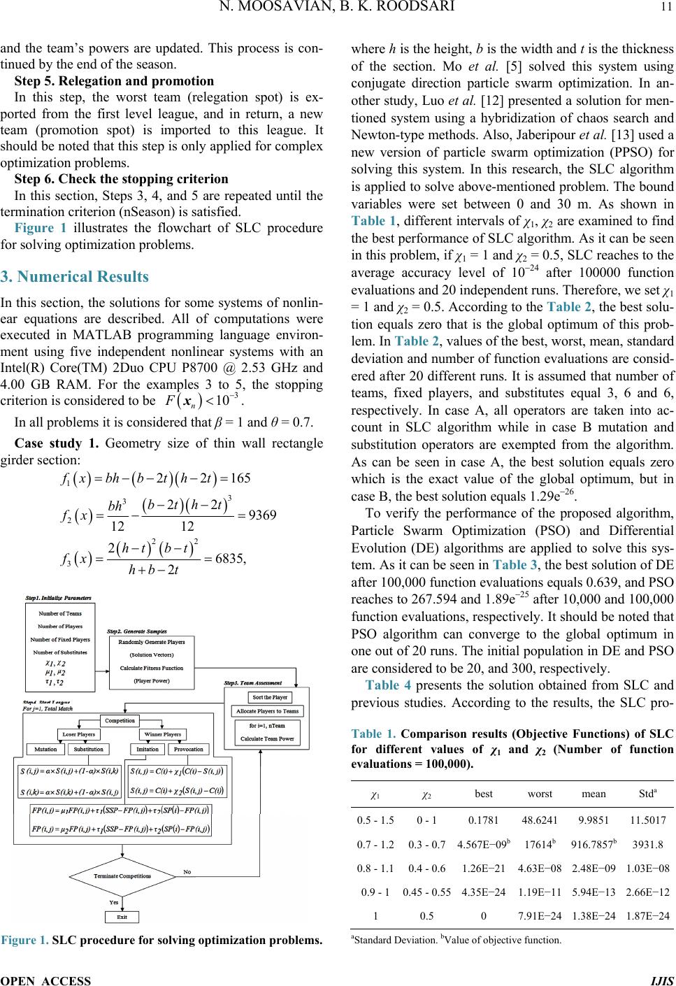 N. MOOSAVIAN, B. K. ROODSARI 11 and the team’s powers are updated. This process is con- tinued by the end of the season. Step 5. Relegation and promotion In this step, the worst team (relegation spot) is ex- ported from the first level league, and in return, a new team (promotion spot) is imported to this league. It should be noted that this step is only applied for complex optimization problems. Step 6. Check the stopping criterion In this section, Steps 3, 4, and 5 are repeated until the termination criterion (nSeason) is satisfied. Figure 1 illustrates the flowchart of SLC procedure for solving optimization problems. 3. Numerical Results In this section, the solutions for some systems of nonlin- ear equations are described. All of computations were executed in MATLAB programming language environ- ment using five independent nonlinear systems with an Intel(R) Core(TM) 2Duo CPU P8700 @ 2.53 GHz and 4.00 GB RAM. For the examples 3 to 5, the stopping criterion is considered to be 3 10 n F x. In all problems it is considered that β = 1 and θ = 0.7. Case study 1. Geometry size of thin wall rectangle girder section: 1 3 3 2 22 3 22165 22 9369 12 12 26835, 2 fxbhbtht btht bh fx htbt fx hb t Figure 1. SLC procedure for solving optimization problems. where h is the height, b is the width and t is the thickness of the section. Mo et al. [5] solved this system using conjugate direction particle swarm optimization. In an- other study, Luo et al. [12] presented a solution for men- tioned system using a hybridization of chaos search and Newton-type methods. Also, Jaberipour et al. [13] used a new version of particle swarm optimization (PPSO) for solving this system. In this research, the SLC algorithm is applied to solve above-mentioned problem. The bound variables were set between 0 and 30 m. As shown in Table 1, different intervals of χ1, χ2 are examined to find the best performance of SLC algorithm. As it can be seen in this problem, if χ1 = 1 and χ2 = 0.5, SLC reaches to the average accuracy level of 1024 after 100000 function evaluations and 20 independent runs. Therefore, we set χ1 = 1 and χ2 = 0.5. According to the Table 2, the best solu- tion equals zero that is the global optimum of this prob- lem. In Table 2, values of the best, worst, mean, standard deviation and number of function evaluations are consid- ered after 20 different runs. It is assumed that number of teams, fixed players, and substitutes equal 3, 6 and 6, respectively. In case A, all operators are taken into ac- count in SLC algorithm while in case B mutation and substitution operators are exempted from the algorithm. As can be seen in case A, the best solution equals zero which is the exact value of the global optimum, but in case B, the best solution equals 1.29e26. To verify the performance of the proposed algorithm, Particle Swarm Optimization (PSO) and Differential Evolution (DE) algorithms are applied to solve this sys- tem. As it can be seen in Table 3, the best solution of DE after 100,000 function evaluations equals 0.639, and PSO reaches to 267.594 and 1.89e25 after 10,000 and 100,000 function evaluations, respectively. It should be noted that PSO algorithm can converge to the global optimum in one out of 20 runs. The initial population in DE and PSO are considered to be 20, and 300, respectively. Table 4 presents the solution obtained from SLC and previous studies. According to the results, the SLC pro- Table 1. Comparison results (Objective Functions) of SLC for different values of χ1 and χ2 (Number of function evaluations = 100,000). χ1 χ2 best worst mean Stda 0.5 - 1.50 - 1 0.1781 48.6241 9.9851 11.5017 0.7 - 1.20.3 - 0.74.567E−09b 17614b 916.7857b3931.8 0.8 - 1.10.4 - 0.61.26E−21 4.63E−08 2.48E−09 1.03E−08 0.9 - 10.45 - 0.554.35E−241.19E−11 5.94E−13 2.66E−12 1 0.5 0 7.91E−24 1.38E−24 1.87E−24 aStandard Deviation. bValue of objective function. OPEN ACCESS IJIS  N. MOOSAVIAN, B. K. ROODSARI 12 Table 2. Reviewing effects of different parameters for SLC in cases A and B. Case A SLC best worst mea n std FCN 3a 6b 6c 0d 7.91E−24 1.38E−24 1.87E−24 10,000 Case A best worst mean std FCN 3 6 6 0 1.87E−24 4.76E−25 4.91E−25 100,000 Case B best worst mean std FCN 3 6 6 1.29E−26 9.25E−25 4.86E−25 3.18E−25 10,000 Case B best worst mean std FCN 3 6 6 5.17E−26 3.32E−24 6.02E−25 7.28E−25 100,000 aNumber of teams. bNumber of fixed players. cNumber of substitutes. dValue of objective function. Table 3. Results of PSO and DE for case study 1. best worst mean std FCN DE 0.639a 3023.6a 663.8763a 949.29 100000 PSO 267.594 10000 9513.4 2176.2 10000 PSO 1.89E−25 10000 8500 3663.5 100000 aValue of objective function. Table 4. Comparison of SLC solutions with other methods in case study 1. Methods B h t f 1(x) f 2(x) f 3(x) SLC 22.057 20.294 2.1705 165 9369 6835 PPSO [8] 43.156 10.129 12.944 709.24 9369 528.04 Mo et al. [11] 8.9431 23.271 12.913 165 9369 529.32 Luo et al. [10] 12.566 22.895 2.7898 166.72 9544.32585.5 vides exact solution and outperforms other discussed methods. Case study 2. Consider 12 ,,, m Ffxfxfxx with 1112 11 1010 109 3512 0 3 5120,2,,9 351 0, iiiii fxxxx fxxxx xi fxxxx The above system has ten unknown variables and ten equations. SLC was used for solving this system. Maximum and minimum of decision variables were set between −1 and 0. In Tables 5 and 6, performance of SLC is verified for different number of players and teams. Values of χ1, χ2 are assumed based on explanations of section 2.1.2 of this paper. Due to the results of both case A and B, the best performance is reached when the number of teams, fixed players, and substitutes are assumed to be 5, 10, Table 5. Reviewing effects of different parameters for SLC in case A. Case Aa SLC Best worst mean std FCN 3 10 10 3.63E−25 1.89E−05 1.49E−06 4.51E−06 10,000 Best worst mean std FCN 5 10 10 9.40E−13 1.06E−06 5.29E−07 2.36E−07 10,000 aSLC with all operators. Table 6. Reviewing effects of different parameters for SLC in case B. Case Ba SLC best worst me a n std FCN 3 10 10 7.64E−31 1.66E+00 1.67E−01 5.25E−01 10000 best worst mean std FCN 5 10 10 4.70E−20 4.76E−12 5.08E−13 1.21E−12 10000 aSLC without mutation and substitution operators. OPEN ACCESS IJIS 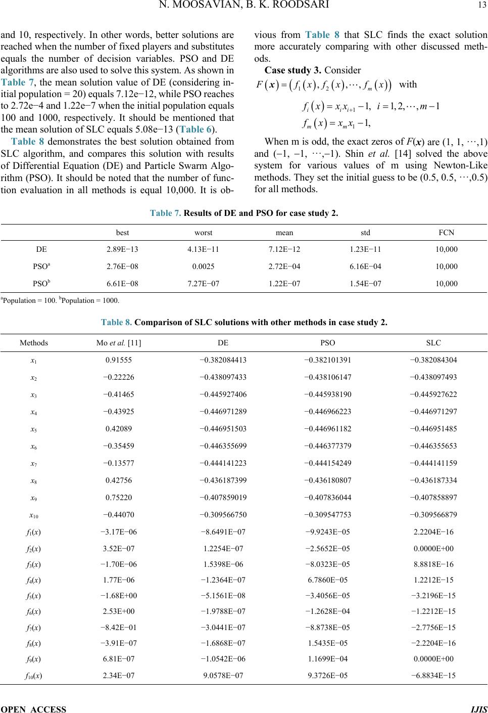 N. MOOSAVIAN, B. K. ROODSARI OPEN ACCESS IJIS 13 vious from Table 8 that SLC finds the exact solution more accurately comparing with other discussed meth- ods. and 10, respectively. In other words, better solutions are reached when the number of fixed players and substitutes equals the number of decision variables. PSO and DE algorithms are also used to solve this system. As shown in Table 7, the mean solution value of DE (considering in- itial population = 20) equals 7.12e−12, while PSO reaches to 2.72e−4 and 1.22e−7 when the initial population equals 100 and 1000, respectively. It should be mentioned that the mean solution of SLC equals 5.08e−13 (Table 6). Case study 3. Consider 12 ,,, m Ffxfxfxx with 1 1 1,1, 2,,1 1, iii mm fx xxim fx xx Table 8 demonstrates the best solution obtained from SLC algorithm, and compares this solution with results of Differential Equation (DE) and Particle Swarm Algo- rithm (PSO). It should be noted that the number of func- tion evaluation in all methods is equal 10,000. It is ob- When m is odd, the exact zeros of F(x) are (1, 1, ···,1) and (1, 1, ···,1). Shin et al. [14] solved the above system for various values of m using Newton-Like methods. They set the initial guess to be (0.5, 0.5, ···,0.5) for all methods. Table 7. Results of DE and PSO for case study 2. best worst mean std FCN DE 2.89E−13 4.13E−11 7.12E−12 1.23E−11 10,000 PSOa 2.76E−08 0.0025 2.72E−04 6.16E−04 10,000 PSOb 6.61E−08 7.27E−07 1.22E−07 1.54E−07 10,000 aPopulation = 100. bPopulation = 1000. Table 8. Comparison of SLC solutions with other methods in case study 2. Methods Mo et al. [11] DE PSO SLC x1 0.91555 −0.382084413 −0.382101391 −0.382084304 x2 −0.22226 −0.438097433 −0.438106147 −0.438097493 x3 −0.41465 −0.445927406 −0.445938190 −0.445927622 x4 −0.43925 −0.446971289 −0.446966223 −0.446971297 x5 0.42089 −0.446951503 −0.446961182 −0.446951485 x6 −0.35459 −0.446355699 −0.446377379 −0.446355653 x7 −0.13577 −0.444141223 −0.444154249 −0.444141159 x8 0.42756 −0.436187399 −0.436180807 −0.436187334 x9 0.75220 −0.407859019 −0.407836044 −0.407858897 x10 −0.44070 −0.309566750 −0.309547753 −0.309566879 f1(x) −3.17E−06 −8.6491E−07 −9.9243E−05 2.2204E−16 f2(x) 3.52E−07 1.2254E−07 −2.5652E−05 0.0000E+00 f3(x) −1.70E−06 1.5398E−06 −8.0323E−05 8.8818E−16 f4(x) 1.77E−06 −1.2364E−07 6.7860E−05 1.2212E−15 f5(x) −1.68E+00 −5.1561E−08 −3.4056E−05 −3.2196E−15 f6(x) 2.53E+00 −1.9788E−07 −1.2628E−04 −1.2212E−15 f7(x) −8.42E−01 −3.0441E−07 −8.8738E−05 −2.7756E−15 f8(x) −3.91E−07 −1.6868E−07 1.5435E−05 −2.2204E−16 f9(x) 6.81E−07 −1.0542E−06 1.1699E−04 0.0000E+00 f10(x) 2.34E−07 9.0578E−07 9.3726E−05 −6.8834E−15 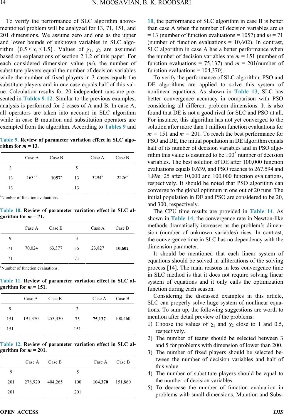 N. MOOSAVIAN, B. K. ROODSARI 14 To verify the performance of SLC algorithm above- mentioned problem will be analyzed for 13, 71, 151, and 201 dimensions. We assume zero and one as the upper and lower bounds of unknown variables in SLC algo- rithm . Values of χ1, χ2 are assumed based on explanations of section 2.1.2 of this paper. For each considered dimension value (m), the number of substitute players equal the number of decision variables while the number of fixed players in 3 cases equals the substitute players and in one case equals half of this val- ue. Calculation results for 20 independent runs are pre- sented in 0.5 1.5 i x Tables 9-12. Similar to the previous examples, analysis is performed for 2 cases of A and B. In case A, all operators are taken into account in SLC algorithm while in case B mutation and substitution operators are exempted from the algorithm. According to Tables 9 and Table 9. Review of parameter variation effect in SLC algo- rithm for m = 13. Case A Case B Case A Case B 3 5 13 13 13 1631a 1057a 13 3294a 2226a aNumber of function evaluations. Table 10. Review of parameter variation effect in SLC al- gorithm for m = 71. Case A Case B Case A Case B 9 3 71 35 71 70,024 63,377 71 23,827 10,602 aNumber of function evaluations. Table 11. Review of parameter variation effect in SLC al- gorithm for m = 151. Case A Case B Case A Case B 9 3 151 75 151 191,370 253,330 151 75,137 100,460 Table 12. Review of parameter variation effect in SLC al- gorithm for m = 201. Case A Case B Case A Case B 9 5 201 100 201 278,920 404,265 201 104,370 151,860 10, the performance of SLC algorithm in case B is better than case A when the number of decision variables are m = 13 (number of function evaluations = 1057) and m = 71 (number of function evaluations = 10,602). In contrast, SLC algorithm in case A has a better performance when the number of decision variables are m = 151 (number of function evaluations = 75,137) and m = 201(number of function evaluations = 104,370). To verify the performance of SLC algorithm, PSO and DE algorithms are applied to solve this system of nonlinear equations. As shown in Table 13, SLC has better convergence accuracy in comparison with PSO considering all different problem dimensions. It is also found that DE is not a good rival for SLC and PSO at all. For instance, this algorithm has not yet converged to the solution after more than 1 million function evaluations for m = 151 and m = 201. To reach the best performance for PSO and DE, the initial population in DE algorithm equals half of its number of decision variables and in PSO algo- rithm this value is assumed to be 100* number of decision variables. The best solution of DE after 100,000 function evaluations equals 0.639, and PSO reaches to 267.594 and 1.89e−25 after 10,000 and 100,000 function evaluations, respectively. It should be noted that PSO algorithm can converge to the global optimum in one out of 20 runs. The initial population in DE and PSO are considered to be 20, and 300, respectively. The CPU time results are provided in Table 14. As shown in Table 14, the convergence rate in Newton-like methods dramatically increases as the problem’s dimen- sion (number of unknown variables) rises. In contrast, the convergence time in SLC has no dependency with the dimension parameter. It should be mentioned that each linear system of equations should be solved in alliterations of the solving process [14]. The main reasons in less convergence time in SLC method is that it does not require solving linear system of equations and it only calls the optimization function during each season. Considering the discussed examples in this article, SLC can properly solve huge system of nonlinear equa- tions. To sum up, the following suggestions are worth to mention after detail preview of the problems: 1) Choose the values of χ1 and χ2 close to 1 and 0.5, respectively. 2) The number of teams should be selected between 3 and 5 for problems with dimension of lower than 200. 3) The number of fixed players should be selected be- tween the number of decision variables and half of this value. 4) The number of substitute players should be equal to the number of decision variables. 5) To decrease the number of function evaluation in problems with small dimensions, Mutation and Subs- OPEN ACCESS IJIS 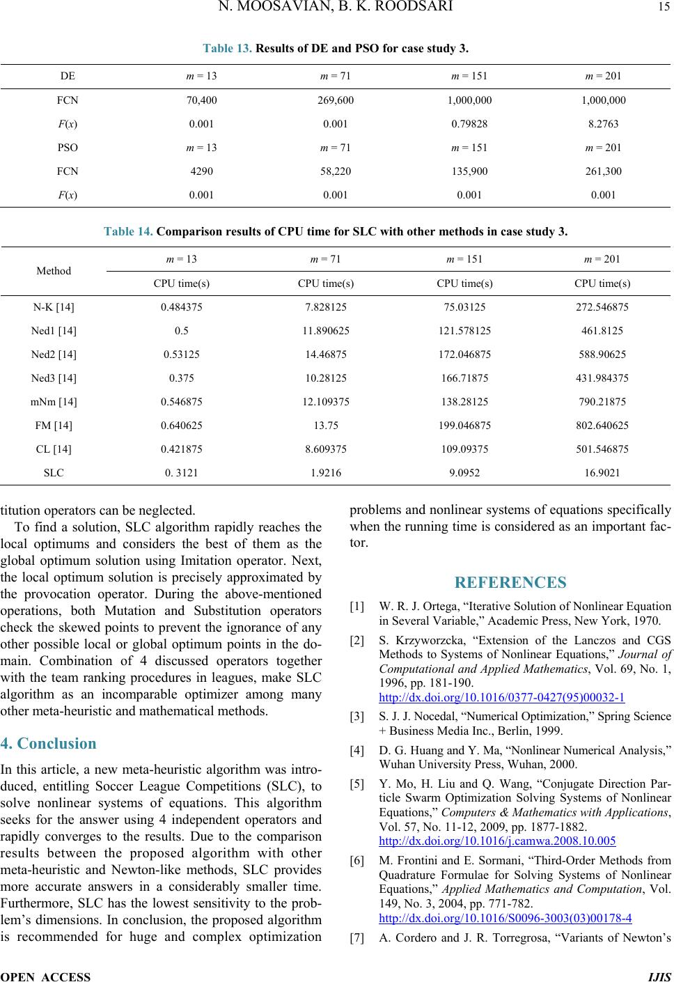 N. MOOSAVIAN, B. K. ROODSARI 15 Table 13. Results of DE and PSO for case study 3. DE m = 13 m = 71 m = 151 m = 201 FCN 70,400 269,600 1,000,000 1,000,000 F(x) 0.001 0.001 0.79828 8.2763 PSO m = 13 m = 71 m = 151 m = 201 FCN 4290 58,220 135,900 261,300 F(x) 0.001 0.001 0.001 0.001 Table 14. Comparison results of CPU time for SLC with other methods in case study 3. m = 13 m = 71 m = 151 m = 201 Method CPU time(s) CPU time(s) CPU time(s) CPU time(s) N-K [14] 0.484375 7.828125 75.03125 272.546875 Ned1 [14] 0.5 11.890625 121.578125 461.8125 Ned2 [14] 0.53125 14.46875 172.046875 588.90625 Ned3 [14] 0.375 10.28125 166.71875 431.984375 mNm [14] 0.546875 12.109375 138.28125 790.21875 FM [14] 0.640625 13.75 199.046875 802.640625 CL [14] 0.421875 8.609375 109.09375 501.546875 SLC 0. 3121 1.9216 9.0952 16.9021 titution operators can be neglected. To find a solution, SLC algorithm rapidly reaches the local optimums and considers the best of them as the global optimum solution using Imitation operator. Next, the local optimum solution is precisely approximated by the provocation operator. During the above-mentioned operations, both Mutation and Substitution operators check the skewed points to prevent the ignorance of any other possible local or global optimum points in the do- main. Combination of 4 discussed operators together with the team ranking procedures in leagues, make SLC algorithm as an incomparable optimizer among many other meta-heuristic and mathematical methods. 4. Conclusion In this article, a new meta-heuristic algorithm was intro- duced, entitling Soccer League Competitions (SLC), to solve nonlinear systems of equations. This algorithm seeks for the answer using 4 independent operators and rapidly converges to the results. Due to the comparison results between the proposed algorithm with other meta-heuristic and Newton-like methods, SLC provides more accurate answers in a considerably smaller time. Furthermore, SLC has the lowest sensitivity to the prob- lem’s dimensions. In conclusion, the proposed algorithm is recommended for huge and complex optimization problems and nonlinear systems of equations specifically when the running time is considered as an important fac- tor. REFERENCES [1] W. R. J. Ortega, “Iterative Solution of Nonlinear Equation in Several Variable,” Academic Press, New York, 1970. [2] S. Krzyworzcka, “Extension of the Lanczos and CGS Methods to Systems of Nonlinear Equations,” Journal of Computational and Applied Mathematics, Vol. 69, No. 1, 1996, pp. 181-190. http://dx.doi.org/10.1016/0377-0427(95)00032-1 [3] S. J. J. Nocedal, “Numerical Optimization,” Spring Science + Business Media Inc., Berlin, 1999. [4] D. G. Huang and Y. Ma, “Nonlinear Numerical Analysis,” Wuhan University Press, Wuhan, 2000. [5] Y. Mo, H. Liu and Q. Wang, “Conjugate Direction Par- ticle Swarm Optimization Solving Systems of Nonlinear Equations,” Computers & Mathematics with Applications, Vol. 57, No. 11-12, 2009, pp. 1877-1882. http://dx.doi.org/10.1016/j.camwa.2008.10.005 [6] M. Frontini and E. Sormani, “Third-Order Methods from Quadrature Formulae for Solving Systems of Nonlinear Equations,” Applied Mathematics and Computation, Vol. 149, No. 3, 2004, pp. 771-782. http://dx.doi.org/10.1016/S0096-3003(03)00178-4 [7] A. Cordero and J. R. Torregrosa, “Variants of Newton’s OPEN ACCESS IJIS  N. MOOSAVIAN, B. K. ROODSARI 16 Method for Functions of Several Variables,” Applied Ma- thematics and Computation, Vol. 183, No. 1, 2006, pp. 199-208. http://dx.doi.org/10.1016/j.amc.2006.05.062 [8] M. T. Darvishi and A. Barati, “Super Cubic Iterative Me- thods to Solve Systems of Nonlinear Equations,” Applied Mathematics and Computation, Vol. 188, No. 2, 2007, pp. 1678-1685. http://dx.doi.org/10.1016/j.amc.2006.11.022 [9] M. T. Darvishi and A. Barati, “A Fourth-Order Method from Quadrature Formulae to Solve Systems of Nonlinear Equations,” Applied Mathematics and Computation, Vol. 188, No. 1, 2007, pp. 257-261. http://dx.doi.org/10.1016/j.amc.2006.09.115 [10] M. T. Darvishi and A. Barati, “A Third-Order Newton- Type Method to Solve Systems of Nonlinear Equations,” Applied Mathematics and Computation, Vol. 187, No. 2, 2007, pp. 630-635. http://dx.doi.org/10.1016/j.amc.2006.08.080 [11] D. K. R. Babajee, et al., “A Note on the Local Conver- gence of Iterative Methods Based on Adomian Decompo- sition Method and 3-Node Quadrature Rule,” Applied Mathematics and Computation, Vol. 200, No. 1, 2008, pp. 452-458. http://dx.doi.org/10.1016/j.amc.2007.11.009 [12] Y.-Z. Luo, G.-J. Tang and L.-N. Zhou, “Hybrid Approach for Solving Systems of Nonlinear Equationsusing Chaos Optimization and Quasi-Newton Method,” Applied Soft Computing, Vol. 8, No. 2, 2008, pp. 1068-1073. http://dx.doi.org/10.1016/j.asoc.2007.05.013 [13] M. Jaberipour, E. Khorram and B. Karimi, “Particle Swarm Algorithm for Solving Systems of Nonlinear Equ- ations,” Computers & Mathematics with Applications, Vol. 62, No. 2, 2011, pp. 566-576. http://dx.doi.org/10.1016/j.camwa.2011.05.031 [14] B. C. Shin, M. T. Darvishi and C.-H. Kim, “A Compari- son of the Newton-Krylov Method with High Order New- ton-Like Methods to Solve Nonlinear Systems,” Applied Mathematics and Computation, Vol. 217, No. 7, 2010, pp. 3190-3198. http://dx.doi.org/10.1016/j.amc.2010.08.051 OPEN ACCESS IJIS
|