 Current Urban Studies 2013. Vol.1, No.4, 110-116 Published Online December 2013 in SciRes (http://www.scirp.org/journal/cus) http://dx.doi.org/10.4236/cus.2013.14012 Open Access 110 The Estimation of Property Tax Capitalisation in the Korean Taxation Context Hyung Min Kim1*, Kyoung-Seok Jang2, Youn-Kyoung Hur3 1Department of Urban Planning and Design, Xianjiaotong-Liverpool University, Suzhou, China 2Office of Economic and Industrial Research, National Assembly Research Service, Seoul, Korea 3Construction Economy Division, Construction and Economy Research Institute of Korea, Seoul, Korea Email: *hm.kim@xjtlu.edu.cn, jangks@assembly.go.kr, ykhur@cerik.re.kr Received August 12th, 2013; revised September 15th, 2013; accepted September 23rd, 2013 Copyright © 2013 Hyung Min Kim et al. This is an open access article distributed under the Creative Commons Attribution License, which permits unrestricted use, distribution, and reproduction in any medium, provided the original work is properly cited. The difference between public services and property tax rates is capitalised into home values. The aim of this research is to estimate the property tax capitalisation rate under a different taxation context of Korea, using a repeat sales method with short-term data on housing prices and estimated tax payments. In the operation of the property taxation, there is complexity that needs to be considered in the estimation of the property tax capitalisation rate. In this research, 32,101 apartment samples in Seoul are used for the anal- ysis. Given these unique institutional circumstances, as a result of the analysis, the property tax capitalisa- tion rate in Seoul was between 73.7% and 82.8% in the analysis periods. Keywords: Housing Prices; Property Tax; Gross Real Estate Tax (GRET); Capitalisation; Repeat Sales Model Introduction The difference between public services and property tax rates is capitalised in home values. This phenomenon is called a capitalisation effect (Yinger et al., 1988; Rosen & Gayer, 2007). Higher property tax payments lead to lower house values if all else being equal. Theoretically, housing prices drop by the dis- counted present value of property tax payments when the prop- erty taxes are imposed. This is called full or complete capi- talisation. However, in the extensive study of Yinger et al. (1988), property taxes were partially capitalised. In spite of a simple concept of property tax capitalisation, it is challenging to estimate the degree of capitalisation (Yinger et al., 1988). Different taxation policy contexts require different analysis methods. During the early 2000s, housing prices increased dras- tically in a selected few areas in Korea. According to a housing price index, housing prices in Seoul increased approximately 50% over the three years in the early 2000s. In response to the changes in the housing market, the Korean government utilised property taxation as a tool to stabilise housing prices and to improve housing affordability. The government announced more than 30 policies on property markets during the period 2003-7 (Jang, 2010: pp. 274-355). Nevertheless, little has been studied about the influence of the reinforced property taxes on housing prices in Korea. Thus, the aim of this research is to estimate the property tax capitalisation rate under a different taxation context of Korea, using a repeat sales method with short-term data on housing prices and estimated tax payments. This study sheds light on the presence of the property tax capitalisation effect and pro- poses a new method to estimate that effect. Institutional Context The Korean government has three hierarchies: the central government, metropolitan governments (si/do, e.g. Seoul, Bu- san or Gyeonggi), and local governments (si/gun/gu). Each government levies property taxes, respectively. In order to cal- culate property tax rates precisely, this section reviews the structure of property taxation in Korea currently being operated in the three levels. Firstly, there are many types of property taxes as a form of a surtax imposed by different levels of governments. These taxes include “Property Tax”1 and “Gross Real Estate Tax (hereafter GRET)” and there are other taxes, based on the same property, such as “City Planning Tax”2, “Local Education Tax”, “Facili- ties Tax”, and “Special Tax for Rural Development”. These taxes should be regarded as one of the property taxes because they are all levied to the same property using the same paying method. For example, when tax payers pay for the “Property Tax” to the local governments, they also have to pay for the “Facilities Tax” to the metropolitan government with the same tax bill. The “Local Education Tax” is additionally imposed to the owner with 20% of property tax payments. These taxes are included in one tax bill so that the governments may collect taxes easily. The collected money is distributed to each gov- ernment. Likewise, the “Special Tax for Rural Development” is the surtax of 20% of the GRET. The GRET is imposed to ex- pensive housing by the central government in order to stabilise housing prices, to recoup capital gains and to contribute to ba- 1In this study, the property tax as a general term is different from the “Prop- erty Tax” as one sort of property taxes in Korea; the property tax includes taxes based on land and property. 2City Planning Tax was incorporated into the part of “Property Tax” in 2011. *Corresponding author.  H. M. KIM ET AL. lanced development between regions. Accordingly, it is easy to underestimate effective property tax rates when tax payers only consider the legal tax rate described in the Local Tax Act. To be precise, all these taxes, thus, need to be regarded as the property taxes. Secondly, the Korean property taxation is progressive by values. Higher tax rates are applied to expensive houses, while lower tax rates, inexpensive ones. Progressiveness was streng- thened due to the enforcement of the “Gross Real Estate Tax Act” in 2006. For houses below 40 million WON3, their “Prop- erty Tax” rate is only 0.15%. However, for houses more expen- sive than 600 million WON, their “Property Tax” rate becomes 1%. If the price is over 2 billion WON, the owner has to pay 2% of assessed housing prices. Ta b le 1 summarises the details of tax rates by housing price bands. Thirdly, local governments have a limited influence in the decision of property tax rates. For the purpose of equity be- tween regions, the “Local Tax Act” bans local governments from changing tax rates. The elastic taxation meant that local governments had the authority to adopt a different tax rate within 50% of flexibility; the elastic tax rates were only oper- ated in 2005 and 2006. During these periods, a few local gov- ernments adopted lower property tax rates than standard tax rates presented in the “Local Tax Act”. However, equity was considered significant and the implementation of elastic taxa- tion ended in 2006. Basically, the central and metropolitan government support the deficit after local governments finance local taxes at given property tax rates. So, there is a discrepancy between burdens of tax payers and benefits from the local gov- ernments. Even though owners of expensive properties pay for a large amount of property taxes on a higher tax rate, they ben- efit from public services similar to those who pay less due to an inflexible tax rate system discussed above. Besides, additional complexity exists in the taxation. A tax payment-cap policy is in operation. The purpose of this policy is to prevent a rapid increase in tax payments caused from sud- den changes in the real estate market. For example, a property tax payment should not exceed over 105% of the last payment when the price of the property is within 300 million WON, 110% for its price is laid between 300 and 600 million WON, and 150%, over 600 million WON. In addition, the aggregate amount of the “Property Tax” and the GRET should not exceed three times of the property tax payments in relation to the cor- responding period last year. This complexity under Korean taxation contexts creates dif- ficulties in estimating the property capitalisation rate. Thus, the principle of the repeat sales model is used to estimate the prop- erty taxation capitalisation. Data and Method Data The Korean central government assesses housing prices of all housing in Korea for tax purpose on a yearly basis viaa gov- ernment agency—Korea Appraisal Board (KAB). The ap- praised prices make it possible to calculate the amount of indi- vidual property tax payments. The unit of the analysis in this research is an individual apartment (high-rise condominium). Extensive data for three years about housing (appraised) prices between 2006 and 2008 Table 1. Legal tax rates and tax base in Korea. Tax title Housing prices (million WON) Tax rate (%) Tax base Below 40 0.15 40 - 100 0.3 Property Tax Over 100 0.5 Assessed housing prices Below 300 1.0 300 - 1400 1.5 1400 - 10,000 2.0 Gross Real Estate Tax 10,000 3.0 Assessed housing prices subtracted 600 million WON City Planning Tax 0.15 The same to the property tax Local Education Tax 20 The amount of property tax Special Tax for Rural Development 20 The amount of global real estate tax Source: The Local Tax Act and Gross Real Estate Tax Act. was used for this research. A sample consists of 32,101 apart- ments, which account for 2.6% of total apartment stocks in Seoul (see Table 2). Apartment is a major housing type in Seoul, accounting for 54.2% of the housing stock (Census in 2005). Almost new housing construction is composed of apart- ments, for example, 76.5% in 2006, and 100% of housing re- newal projects were a form of high-rise apartments (Ha, 2010). Thus, the sample of this research is large enough to represent Seoul’s housing market. The average housing price was 222,375 thousand WON in 2006, 279,042 thousand WON in 2007 (a 25.5% increase in relation to 2006), and 290,946 thousand WON in 2008 (a 4.3% increase in relation to 2007). More details are in Appendix. To calculate the amount of tax payments and effective tax rates, following four factors were considered in the Korean context: appraised apartment prices, tax-rate bands, the elastic tax rates in 2006, and the property tax payment cap4. These factors made the amount of property tax payments change every year. The effective tax rate is house’s property tax pay- ment divided by its market value (Yinger et al., 1988). The summary of calculated tax payment and their effective tax rates are presented in Table 3. Based on aggregated tax payments and appraised prices, ef- fective property tax rates were 2.059 mill in 2006, 1.990 mill in 2007, and 2.139 mill in 2008, respectively. Methodology This study takes advantage of the principle of a repeat sales model. The repeat sales model was developed by Bailey et al. (1963). Then, Case & Shiller (1987) used this model to estimate variations in housing prices and to create an housing price in- 4The “Local Tax Act” bans local governments from elastic tax rates across regions for the purpose of equity. The elastic taxation was that local gov- ernments had the authority to adopt a different tax rate within fifty per cent of flexibility; the elastic tax rates were only operated in 2005 and 2006. During this period, a few local governments adopted lower property tax rates than standard tax rates presented in the “Local Tax Act”. The central and metropolitan government support the deficit after local governments finance local taxes. 3US $1 = 956 WON in 2006, 1103 WON in 2008. Open Access 111  H. M. KIM ET AL. Table 2. Statistics of summary1. Variables Mean Standard deviation Minimum Maximum The age of house in 2006 11.86 7.23 0.00 39.00 House net area (m2) 72.70 24.29 23.70 244.97 Housing price in 20062 222.38 164.21 38.00 2780.00 Housing price in 20072 279.04 222.08 39.00 3856.00 Housing price in 20082 290.95 208.57 48.00 3480.00 1Number of samples is 32101; 2Million WON. Table 3. Estimated effective tax rates and tax payments by districts. Tax rates (mill) Tax payment per house (thousand WON) 2006 2007 2008 2006 2007 2008 Gangnam 2.243 2.483 3.085 1360 20842660 Gangdong 2.189 2.078 2.286 616 754 827 Gangbuk 1.814 1.704 1.662 283 314 369 Gangseo 1.830 1.643 1.769 312 386 424 Gwanak 1.968 1.840 1.902 373 417 466 Gwangjin 2.517 2.318 2.535 739 914 1018 Guro 1.841 1.714 1.727 299 338 385 Geumcheon 2.106 1.967 2.014 337 370 409 Nowon 1.743 1.603 1.613 256 291 336 Dobong 2.058 1.944 1.926 325 357 406 Dongdaemun 2.059 1.997 2.020 424 459 517 Dongjak 2.181 1.981 2.091 538 629 714 Mapo 2.184 2.017 2.154 548 638 715 Seodaemun 2.310 2.219 2.250 454 490 546 Seocho 2.643 3.057 3.795 1,439 22852845 Seongdong 2.427 2.274 2.397 643 729 808 Seongbuk 1.993 1.928 1.945 386 419 473 Songpa 2.190 2.314 2.774 969 14141700 Yangcheon 1.991 1.870 2.166 545 825 954 Yeongdeungpo 2.129 2.058 2.210 585 769 890 Yongsan 2.658 2.828 3.196 1248 19182334 Eunpyeong 2.139 2.030 2.056 352 379 421 Jongno 1.999 1.965 2.014 428 490 565 Jung 1.959 1.902 2.079 558 652 719 Jungnang 2.062 1.946 1.974 311 340 378 Average (Seoul) 2.059 1.990 2.139 534 698 808 Note: Mill is 1/1000. dex using transaction prices. Since Bailey et al. and Case & Shiller, the repeat sales model has been widely used in generat- ing a housing price index and understanding property markets (McMillen, 2008). The principle of the repeat sales model is that, when one house is transacted, the price matches to the previous transaction price of the same house so that the differ- ence between the two prices can be measured precisely. The changes in housing prices are estimated by a regression analysis. The rationale of this matching is to remove any expected biases. Every single house has its unique locational and structural cha- racteristics. Accordingly, only when the house is compared to the same house without any structural alterations, can real changes of housing prices be correctly measured. The repeat sales model adds time-variables to the hedonic price model used for a cross-sectional analysis. As the same house is compared in calculation of housing price changes, the repeat sales model rules out the effects of other variables, such as lot size, bedrooms, toilets, and garages, as long as the house was not renovated between the two transaction periods. In the model of the initial repeat sales model by Bailey et al. (1963), a natural log was taken to calculate the changing rates of housing prices. The natural log makes left-sides directly a variation rate in housing prices. Pf is the first transaction and Ps is the second one in Equations (1) and (2) (Choi et al., 2010). and are the intercept composed of macro-economic factors, housing preferences and other factors that can influence housing prices. ,, 1 In In K isis s s i PX (1) ,, 1 In In K ifif f f i PX (2) where Xi is characteristic of the house. i is coefficient. and are error terms. As Equation (1) subtracts Equation (2), the equation is sim- plified to conduct a regression analysis. In Equation (3), the explanatory variables in a general hedonic price model are de- leted. 1 In v T s tt t f PD P (3) where, 10, v f ee . The left side is the rate of variations in housing prices; all in- dividual housing characteristics are removed in the right side. This is the most advantageous feature in the repeat sales model simplifying model specification. Dt in Equation (3) is a dummy variable. It becomes one when transaction occurs, otherwise zero. βt is the coefficient to be estimated by conducting a re- gression analysis. βt can be transformed to a housing price in- dex5. McMillen (2003) and Kim & Lee (2004, 2005) modify the repeat sales model. They divide variables into time-varying variables and time-fixed variables to discover how influence of the time-varying variables has changed, by estimating the coef- ficient of the time-varying variables, where time-fixed variables are eliminated. Likewise, this paper utilises the principle of the repeat sales model to estimate the property tax capitalisation effect under the Korean taxation context6. 5 exp 100 tt I . 6Although this research uses appraisal prices, the principle of the analysis relies on the repeat sales model that use transaction data. Open Access 112  H. M. KIM ET AL. When there are no property taxes, the hedonic price model can be specified like Equation (4). 01 ˆK kt k P X (4) where, is the housing price before imposing the property tax. ˆ P X is attributes of the house. 0 is an intercept. k is a coefficient. When the effective property tax rate is , the amount of property taxes is P P. should be divided by the dis- count rate (r) in order to acquire the total present value of prop- erty taxes. When the property tax is in operation, the hedonic price model can be expressed like Equation (5)7. 1 1 Kt tkt k T PX r (5) In Equation (5), 1t Tr is a net present value of property tax payments and β is a coefficient that indicates the capitalisation rate. If β equals one, property taxes are fully capitalised. Hous- ing prices decrease by the present value of increased property taxes. On the other hand, ifequals zero, housing prices do not change regardless of newly added property taxes. In Equation (5), the period of the left side—the housing price (P)—is t while, on one of the right side—the amount of property tax (T) —is t − 1. Pt is closely tied to 1t P as effective tax rates and the amount of total property taxes are decided by housing prices, causing an auto-correlation problem that creates difficulty in estimating by OLS. Due to the Korean taxation context dis- cussed in the Section 2, one more step is required. In order to remove the auto-correlation problem, the repeat sales method is modified as suggested by McMillen (2003) and used by Kim & Lee (2005). In the period t + 1, housing prices including prop- erty taxes become Equation (6). 11 1 Kt tt kt k T PX r (6) If Equation (6) is subtracted from Equation (5), the attributes of the house are eliminated. It is possible when there have been no substantial physical changes to housing attributes between t and t + 1. Finally, Equation (7) can be reached to a simplified form to conduct a regression analysis. 101tt tt PP TT 1 0 (7) is 1tt , and this intercept signifies changes of hous- ing prices due to the socio-economic conditions such as income levels, the demand for or the supply of housing, public services and employment. These factors are not spatially specific, thus can be equally applied to all areas in Seoul. 1 is the coeffi- cient that represents the change in housing prices caused by the changes of property taxes. 1 equals r , therefore, is calculated by 1r . In addition to the changes in market trends such as the de- mand and the supply, local influences caused by location-spe- cific changes in amenity, infrastructure, and accessibility, can differ between districts over the analysis period. For example, the construction of an outer circular highway around Seoul was completed in 2006. Due to the new highway, accessibility was improved in the northern part of Seoul, which influenced hous- ing prices. Housing supply varies between districts. For exam- ple, while there was no new apartment construction in Nowon, 27,559 new apartments were built in Songpa in 2007-2008. Conditions of supply and demand in each region create a dis- crepancy in housing price movements. It is necessary to con- sider these effects are different in each district. Thus, district dummy variables are added to Equation (4) to measure the lo- cation-specific influence over time. For example, for Seochogu, only the Seochogu’s district dummy variable equals one, other- wise zero. District dummy variables explain time-varying ef- fects between districts. Result of Analysis As a result of a regression analysis8, almost all variables are statistically significant at the 95% confidence level (see Table 4). The intercept—17,537—plays an important role in inter- preting the trend in the housing market. With taxation effects and location-specific differences controlled, the intercept ex- plains that housing prices increased by 17,537 thousand WON on average between 2007 and 2008. When referring to the av- erage housing price in 2007, the average change in housing prices over the one year was a 6.3% increase (=17.537/279.04). This is attributable to the provision of public goods, macro- economic factors, and the demand for and the supply of hous- ing. Only four district dummy variables are not significant at the 5% significance level, but two of them are statistically signifi- cant at the 90% confidence level (see Ta b l e 5 )9. Two districts, Eunpyeong and Gwanak, show that the dummy variable is not significant at the 10% of the significance level. This is due to variations in housing prices from house to house in Eunpyeong and Gwanak are so large that the statistics cannot conclude that the change in housing prices is different from the base district, Gangnam. For example, there have been redevelopment pro- jects, called New Town Development, in Eunpyeo ng, since 2002. Thus the infrastructure provided concentrated on specific areas. This caused larger variations in housing prices in Eun- pyeong. Housing prices in the new residential development in Eunpyeong increased much more than outside of the develop- 7Theoretically, capitalisation takes place at the time of the announcement o the tax change. However, one year time lag is necessary given the policy context. Property taxation is complicated enough to recognise because they consist of different kinds of taxes in Korea. In addition, the amount of prop- erty taxes is billed to home owners in June and September whereas apprais- ing is done in January and noticing, in April. Thus, this study assumes that property taxes in year t have an influence on housing prices in year t + 1, taking a one-year time-lag in Equation (5). The assumption about the one-year time-lag is reasonable as far as processes of appraisal, notice, and billing are concerned. Jan Apr Jun Sep Jan AppraisalNotice landlords of housing prices Billing property taxesBilling property taxesAppraisal Year tYear t+1 Capitalisation 8This model has 48.3% of explanatory power. The low R-square is the weakness of repeat sales model because the repeat sales model does not have other independent variables that can explain the variation in the de- pendent variable. 9The regression is based on housing prices changes from 2007 to 2008. Due to the one-year time-lag, changes from 2006 to 2007 were not analysed in this regression analysis. Open Access 113  H. M. KIM ET AL. Table 4. Descriptive statistics of dependent and independent variables. Variables Mean Standard Deviation Minimum Maximum Tax payment (independent variable) Tt − Tt−1 163.7 502.0 −1,785.7 13,819.2 Housing price (dependent variable) Pt+1 − Pt 11,904 25,801 −376,000 239,000 Note: Unit is thousand WON. Table 5. Result of a regression analysis. Coeffici ent Standard Eerror t-value p-value Intercept 17537.0 475.5 36.88 <.0001 ∆T −21.9 0.2 −94.70 <.0001 Gangdong −20226.0 647.7 −31.23 <.0001 Gangbuk 19625.0 846.6 23.18 <.0001 Gangseo −15055.0 680.5 −22.12 <.0001 Gwanak 354.5 753.9 0.47 .6381 Gwangjin −12842.0 886.5 −14.49 <.0001 Guro 6217.5 656.3 9.47 <.0001 Geumcheon −2891.6 818.5 −3.53 .0004 Nowon 6328.7 531.9 11.90 <.0001 Dobong 7193.4 607.1 11.85 <.0001 Dongdaemun 8000.8 740.9 10.80 <.0001 Dongjak 2530.7 771.5 3.28 .0010 Mapo −5103.7 810.4 −6.30 <.0001 Seodaemun 3538.1 783.6 4.52 <.0001 Seocho −13922.0 724.6 −19.21 <.0001 Seongdong −2322.8 700.2 −3.32 .0009 Seongbuk 7708.3 690.7 11.16 <.0001 Songpa −24975.0 613.9 −40.68 <.0001 Yangcheon −31276.0 684.4 −45.70 <.0001 Yeongdeungpo 1195.8 691.5 1.73 .0838 Yongsan 31316.0 1023.7 30.59 <.0001 Eunpyeong 483.0 958.8 0.50 .6144 Jongno 8174.7 1490.7 5.48 <.0001 Jung −16302.0 1184.0 −13.77 <.0001 Jungnang −1398.6 735.6 −1.90 .0573 *Dependent variable: Pt+1 − Pt; **adj-R square: 0.4831; ***Notes: The unit is thousand WON, and Gangnam is the basement of district-dummy-variables. ment area10. Yongsan has the highest dummy-variable coeffi- cient. Yongsan is in the middle of the three central business districts in Seoul, but the quality of houses is in general not as good as other residential areas. Recently, there have been rede- velopment projects all over the Yongsan area. The dummy va- riable reflects the effect of the projects on housing price changes in Yongsan. Yangcheon and Songpa show the biggest decrease in housing prices. These two districts including Gangnam belonged to the most expensive areas in Seoul. Housing prices on the expensive areas decreased the most be- tween 2007 and 2008. The coefficient 1 is –21.868. This figure represents that housing prices decreased by 21.868 thousand WON when the property tax increased by one thousand WON. If there was no change in property tax payments, housing prices would increase by 17,537 (the intercept, 0 ) thousand WON. Housing prices decreased by 17,515 WON (17,537 – 21.868 × 163.7) on aver- age due to the increase in property taxes. The property tax capitalisation rate, β is estimated using es- timated coefficient 1 . The capitalisation rate can be acquired by multiplying 1 by the discount rate. The discount rate is an opportunity cost that the home-owners can accrue when they invest in other options instead of housing. Simply, the long- term interest rate could be used as the discount rate (DiPasquale & Wheaton, 1996: p. 207). However, deciding on a discount rate has been problematic in estimating the property tax capi- talisation rate (Yinger et al., 1988). Some studies adopt a nomi- nal discount rate instead of a real discount rate and some use higher rates than the real rates, thus making the capitalisation rate higher. A real discount rate needs to be used and income tax on interest and tax deduction should be considered when measuring the real discount rate (Yinger et al., 1988). Accord- ing to the Bank of Korea, the long-term interest rate was 3.98% in 2006 and 4.47% in 2007. The income tax rate on interest income was 15.4%. Considering the income tax rate on the interest, the real discount rate becomes 3.37% and 3.78%, re- spectively. Accordingly, the capitalisation rate of the property taxes becomes 73.7% and 82.8%. Thus, it is reasonable to con- clude that the degree of property tax capitalisation was some- where between 73.7% and 82.8% (see Ta bl e 6 ). As studied by Yinger et al. (1988), the result shows partial capitalisation that means the effect could transfer to the future owner (Palmon & Smith, 1998) or to tenants thus resulting in an increase in rents. Conclusion This paper focuses on the property tax capitalisation effect under a unique Korean taxation context. The model employed in this research is simple but based on reasonable assumption in which the time-fixed variables can be eliminated. While a con- ventional hedonic price model includes locational and structural variables, the modified repeat sales model utilises variations in property tax payments, which simplifies model specification. The model in this research used three years data on housing prices and tax payments. Given these unique institutional circumstances, as a result of the analysis, the property tax capitalisation rate in Seoul was between 73.7% and 82.8% in the period 2007-8. This is partial 10There are two residential new development plans in Eunpyeong. An in- crease in housing prices on average in the areas within the development is 11.2 (million WON) while outside of the development is 10.1 (million WON). This shows that there exists a heterogeneous housing market even in the same district. Open Access 114 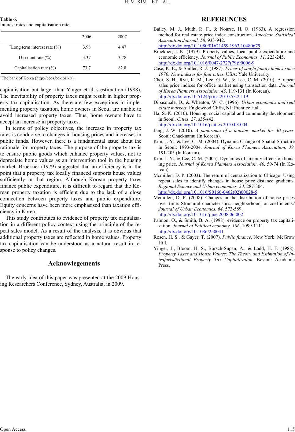 H. M. KIM ET AL. Open Access 115 Table 6. Interest rates and capitalisation rate. 2006 2007 +Long term interest rate (%) 3.98 4.47 Discount rate (%) 3.37 3.78 Capitalisation rate (%) 73.7 82.8 +The bank of Korea (http://ecos.bok.or.kr/). capitalisation but larger than Yinger et al.’s estimation (1988). The inevitability of property taxes might result in higher prop- erty tax capitalisation. As there are few exceptions in imple- menting property taxation, home owners in Seoul are unable to avoid increased property taxes. Thus, home owners have to accept an increase in property taxes. In terms of policy objectives, the increase in property tax rates is conducive to changes in housing prices and increases in public funds. However, there is a fundamental issue about the rationale for property taxes. The purpose of the property tax is to ensure public goods which enhance property values, not to depreciate home values as an intervention tool in the housing market. Bruekner (1979) suggested that an efficiency is in the point that a property tax locally financed supports house values sufficiently in that region. Although Korean property taxes finance public expenditure, it is difficult to regard that the Ko- rean property taxation is efficient due to the lack of a close connection between property taxes and public expenditure. Equity concerns have been more emphasised than taxation effi- ciency in Korea. This study contributes to evidence of property tax capitalisa- tion in a different policy context using the principle of the re- peat sales model. As a result of the analysis, it is obvious that additional property taxes are reflected in home values. Property tax capitalisation can be understood as a natural result in re- sponse to policy changes. Acknowlegements The early idea of this paper was presented at the 2009 Hous- ing Researchers Conference, Sydney, Australia, in 2009. REFERENCES Bailey, M. J., Muth, R. F., & Nourse, H. O. (1963). A regression method for real estate price index construction. American Statistical Association Journal, 58, 933-942. http://dx.doi.org/10.1080/01621459.1963.10480679 Bruekner, J. K. (1979). Property values, local public expenditure and economic efficiency. Journal of Public Economics, 11, 223-245. http://dx.doi.org/10.1016/0047-2727(79)90006-9 Case, K. E., & Shiller, R. J. (1987). Prices of single family homes since 1970: New indexes for four cities. USA: Yale University. Choi, S.-H., Ryu, K.-M., Lee, G.-W., & Lee, C.-M. (2010). A repeat sales price indices for office market using transaction data. Journal of Korea Planners Association, 45, 119-131 (In Korean). http://dx.doi.org/10.5124/jkma.2010.53.2.119 Dipasquale, D., & Wheaton, W. C. (1996). Urban economics and real estate markets. Englewood Cliffs, NJ: Prentice Hall. Ha, S.-K. (2010). Housing, social capital and community development in Seoul. Cities, 27, s35-s42. http://dx.doi.org/10.1016/j.cities.2010.03.004 Jang, J.-W. (2010). A panorama of a housing market for 30 years. Seoul: Chaeknamu (In Korean). Kim, J.-Y., & Lee, C.-M. (2004). Dynamic Change of Spatial Structure in Seoul: 1993-2004. Journal of Korea Planners Association, 39, 191-205 (In Korean). Kim, J.-Y., & Lee, C.-M. (2005). Dynamics of amenity effects on hous- ing price. Journal of Korea Planners Association, 40, 59-74 (In Ko- rean). Mcmillen, D. P. (2003). The return of centralization to Chicago: Using repeat sales to identify changes in house price distance gradients. Regional Science and Urban economics, 33, 287-304. http://dx.doi.org/10.1016/S0166-0462(02)00028-5 Mcmillen, D. P. (2008). Changes in the distribution of house prices over time: Structural characteristics, neighborhood, or coefficients? Journal of Urban Economics, 64, 573-589. http://dx.doi.org/10.1016/j.jue.2008.06.002 Palmon, O., & Smith, B. A. (1998). evidence on property tax capitali- zation. Journal of Political economy, 106, 1099-1111. http://dx.doi.org/10.1086/250041 Rosen, H. S., & Gayer, T. (2007). Public finance. New York: McGrow Hill. Yinger, J., Bloom, H. S., Börsch-Supan, A., & Ladd, H. F. (1988). Property Taxes and House Values: The Theory and Estimation of In- trajurisdictional Property Tax Capitalization. Boston: Academic Press. 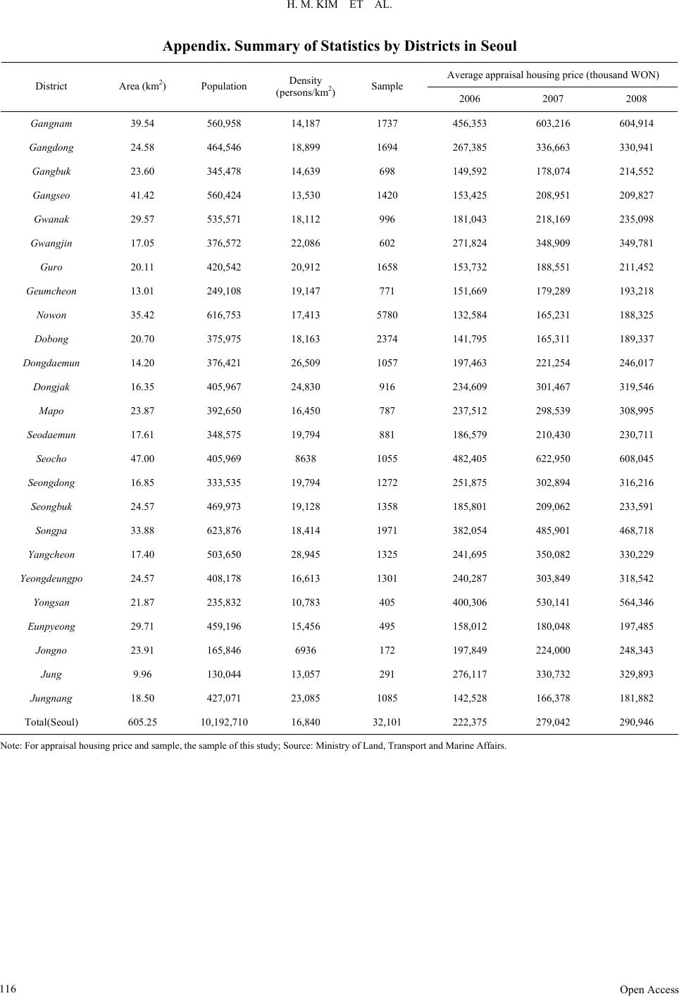 H. M. KIM ET AL. Appendix. Summary of Statistics by Districts in Seoul Average appraisal housing price (thousand WON) District Area (km2) Population Density (persons/km2) Sample 2006 2007 2008 Gangnam 39.54 560,958 14,187 1737 456,353 603,216 604,914 Gangdong 24.58 464,546 18,899 1694 267,385 336,663 330,941 Gangbuk 23.60 345,478 14,639 698 149,592 178,074 214,552 Gangseo 41.42 560,424 13,530 1420 153,425 208,951 209,827 Gwanak 29.57 535,571 18,112 996 181,043 218,169 235,098 Gwangjin 17.05 376,572 22,086 602 271,824 348,909 349,781 Guro 20.11 420,542 20,912 1658 153,732 188,551 211,452 Geumcheon 13.01 249,108 19,147 771 151,669 179,289 193,218 Nowon 35.42 616,753 17,413 5780 132,584 165,231 188,325 Dobong 20.70 375,975 18,163 2374 141,795 165,311 189,337 Dongdaemun 14.20 376,421 26,509 1057 197,463 221,254 246,017 Dongjak 16.35 405,967 24,830 916 234,609 301,467 319,546 Mapo 23.87 392,650 16,450 787 237,512 298,539 308,995 Seodaemun 17.61 348,575 19,794 881 186,579 210,430 230,711 Seocho 47.00 405,969 8638 1055 482,405 622,950 608,045 Seongdong 16.85 333,535 19,794 1272 251,875 302,894 316,216 Seongbuk 24.57 469,973 19,128 1358 185,801 209,062 233,591 Songpa 33.88 623,876 18,414 1971 382,054 485,901 468,718 Yangcheon 17.40 503,650 28,945 1325 241,695 350,082 330,229 Yeongdeungpo 24.57 408,178 16,613 1301 240,287 303,849 318,542 Yongsan 21.87 235,832 10,783 405 400,306 530,141 564,346 Eunpyeong 29.71 459,196 15,456 495 158,012 180,048 197,485 Jongno 23.91 165,846 6936 172 197,849 224,000 248,343 Jung 9.96 130,044 13,057 291 276,117 330,732 329,893 Jungnang 18.50 427,071 23,085 1085 142,528 166,378 181,882 Total(Seoul) 605.25 10,192,710 16,840 32,101 222,375 279,042 290,946 Note: For appraisal housing price and sample, the sample of this study; Source: Ministry of Land, Transport and Marine Affairs. Open Access 116
|