Urban Greening Using an Intelligent Multi-Objective Location Modelling with Real Barriers: Towards a Sustainable City Planning

doi:10.4236/cus.2013.14008

Paper Menu >>

Journal Menu >>

Current Urban Studies

2013. Vol.1, No.4, 75-86

Published Online December 2013 in SciRes (http://www.scirp.org/journal/cus) http://dx.doi.org/10.4236/cus.2013.14008

Open Access 75

Urban Greening Using an Intelligent Multi-Objective

Location Modelling with Real Barriers: Towards

a Sustainable City Planning

Meher Niga r N e ema1*, Khandoker Md. Maniruzzaman2, Akira Ohgai3

1Department of Urban and Regional Plannin g , Bangladesh University of

Engineering and Techno l o g y, Dhaka, Bangladesh

2Department of Urban and Regional Planning, College of Architectu re Planning,

University of Dammam, Dammam, KSA

3Department of Architecture and Civil Engineering, Toyohashi University of Tec h n ol o gy, Toyohashi, J ap a n

Email: *mnnneema@yahoo.com

Received May 22nd, 2013; revised Jun e 28 th, 2013; accepted July 15th, 2013

mons Attribution License, which permits unrestricted use, distribution, and reproduction in any medium, pro-

vided the original work is properly cited.

Greenery is one of the important ingredients for urban planning with a sustainable environment. Increas-

ing parks and open spaces (POS) to offer a greater diversity of green spaces have substantial impact on its

environment in many mega cities around the world. However, any place cannot be a potential site for POS

due to multi-objective modeling nature of POS planning. In this paper, an intelligent multi-objective con-

tinuous optimization model is thus developed for locating POS with particular emphasis on greeneries

that will potentially benefit and facilitate the planning of a sustainable city. Three environmentally inc-

ommensurable factors analyzed with the help of geographic information systems (GIS) namely air-quality,

noise-level, and population-distribution have been considered in the model and a genetic algorithm (GA)

is used to solve the continuous optimization problem heuristically. The model has been applied to Dhaka

city as a case study to find the optimal locations of additional POS to make it a sustainable city by ame-

liorating its degraded environment. The multiple objectives are combined into a single one by employing

a dynamic weighting scheme and a set of non-dominated Pareto optimal solutions is derived. The ob-

tained alternative non-dominated solutions from the robust modelling approach can serve as a candidate

pool for the city planners in decision making for POS planning by selecting an alternative solution which

is best suited for the prevailing land-use pattern in a city. The model has successfully demonstrated to

provide optimal locations of new POS. In addition, we found that locations of POS can be optimized even

by integrating it with land cover and uses like lakes, streams, trails (for simplicity which were considered

as a barrier constraint in the model) to rejuvenate added beauties in a city. The obtained results thus indi-

cate that the developed multi-objective POS location model can serve as an effective tool for urban POS

planning maintaining sustainable environment.

Keywords: Urban Greening; Parks and Open Space; Sustainable Environment; GA and GIS; Intelligent

Location Modelling

Introduction

In an integral urban planning, greeneries can predominantly

be found in parks, playgrounds, gardens etc. Parks and open

spaces (POS) i.e. greeneries in particular can substantially im-

prove the livability of land uses and city environment. Its im-

portant functions are: 1) potential amelioration of microclimate,

2) absorbtion of pollutants, 3) reduction of noise levels includ-

ing a significant improvement of the lifestyle of city-dwellers

by allowing admixture with nature and promoting social inter-

actions (Schipperijn et al., 2010; Szeremeta et al., 2009; Gob-

ster, 1998; Morancho, 2003; Uy & Nakagoshi, 2008; Chiesura,

2004; Egger, 2006; Kong et al., 2010; Borrego et al., 2006;

Lam, 2005; Poggio & Vrcaj, 2009; Nordh et al., 2009; BenDor

et al., 2013; Choumert, 2010; Neema et al., 2013; Neema &

Ohgai, 2013; Neema et al., 2008). Importantly, the necessity of

POS in landscape planning and design can be realized in

densely populated cities around the globe (Lam et al., 2005).

As such a densely populated city, Dhaka has emerged as a

fast growing mega-city. In 1975, it started with a population of

only 2.2 million which has culminated to 16 million in 2010. In

2015, a predicted population is 21 million. It can be envisaged

that due to this rapid growth of population in Dhaka, it is con-

fronted with a big challenge to deal with serious environmental

degradation due mainly to the significantly diminished number

of POS. Once, Dhaka city was considered as a green city but

now it has left with only 21.6% open space (but not green

spaces) of its total area with huge population (SDNP, 2005).

Statistically, it can be calculated that only approximately 8 sq.

meter POS is available per person in Dhaka city (Uddin, 2005),

which is rather insufficient for a healthy sustainable city. In

*Corresponding author.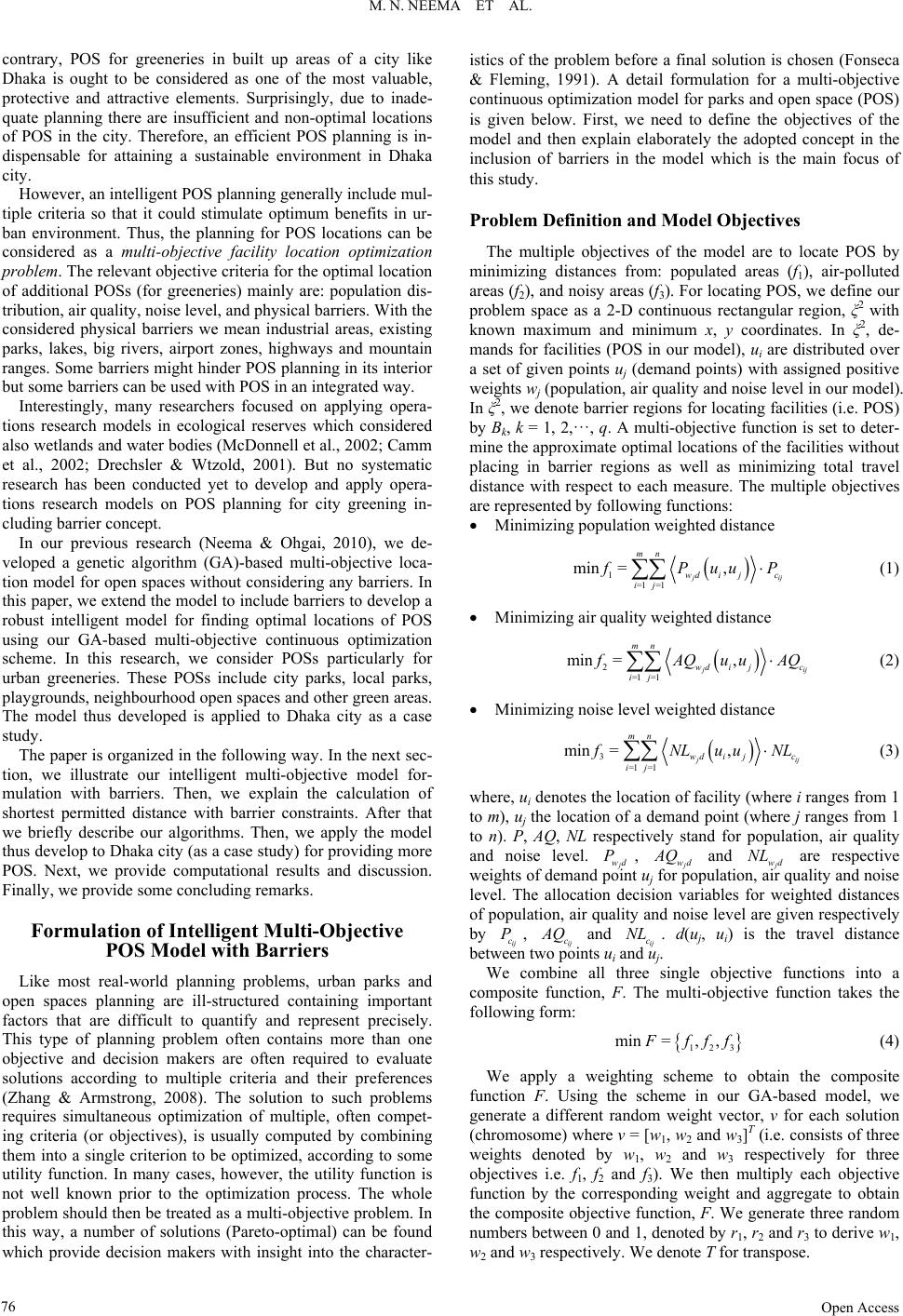

M. N. NEEMA ET AL.

contrary, POS for greeneries in built up areas of a city like

Dhaka is ought to be considered as one of the most valuable,

protective and attractive elements. Surprisingly, due to inade-

quate planning there are insufficient and non-optimal locations

of POS in the city. Therefore, an efficient POS planning is in-

dispensable for attaining a sustainable environment in Dhaka

city.

However, an intelligent POS planning generally include mul-

tiple criteria so that it could stimulate optimum benefits in ur-

ban environment. Thus, the planning for POS locations can be

considered as a multi-objective facility location optimization

problem. The relevant objective criteria for the optimal location

of additional POSs (for greeneries) mainly are: population dis-

tribution, air quality, noise level, and physical barriers. With the

considered physical barriers we mean industrial areas, existing

parks, lakes, big rivers, airport zones, highways and mountain

ranges. Some barriers might hinder POS planning in its interior

but some barriers can be used with POS in an integrated way.

Interestingly, many researchers focused on applying opera-

tions research models in ecological reserves which considered

also wetlands and water bodies (McDonnell et al., 2002; Camm

et al., 2002; Drechsler & Wtzold, 2001). But no systematic

research has been conducted yet to develop and apply opera-

tions research models on POS planning for city greening in-

cluding barrier concept.

In our previous research (Neema & Ohgai, 2010), we de-

veloped a genetic algorithm (GA)-based multi-objective loca-

tion model for open spaces without considering any barriers. In

this paper, we extend the model to include barriers to develop a

robust intelligent model for finding optimal locations of POS

using our GA-based multi-objective continuous optimization

scheme. In this research, we consider POSs particularly for

urban greeneries. These POSs include city parks, local parks,

playgrounds, neighbourhood open spaces and other green areas.

The model thus developed is applied to Dhaka city as a case

study.

The paper is organized in the following way. In the next sec-

tion, we illustrate our intelligent multi-objective model for-

mulation with barriers. Then, we explain the calculation of

shortest permitted distance with barrier constraints. After that

we briefly describe our algorithms. Then, we apply the model

thus develop to Dhaka city (as a case study) for providing more

POS. Next, we provide computational results and discussion.

Finally, we provide some concludi ng remarks .

Formulation of Intelligent Multi-Objective

POS Model with Barriers

Like most real-world planning problems, urban parks and

open spaces planning are ill-structured containing important

factors that are difficult to quantify and represent precisely.

This type of planning problem often contains more than one

objective and decision makers are often required to evaluate

solutions according to multiple criteria and their preferences

(Zhang & Armstrong, 2008). The solution to such problems

requires simultaneous optimization of multiple, often compet-

ing criteria (or objectives), is usually computed by combining

them into a single criterion to be optimized, according to some

utility function. In many cases, however, the utility function is

not well known prior to the optimization process. The whole

problem should then be treated as a multi-objective problem. In

this way, a number of solutions (Pareto-optimal) can be found

which provide decision makers with insight into the character-

istics of the problem before a final solution is chosen (Fonseca

& Fleming, 1991). A detail formulation for a multi-objective

continuous optimization model for parks and open space (POS)

is given below. First, we need to define the objectives of the

model and then explain elaborately the adopted concept in the

inclusion of barriers in the model which is the main focus of

this study.

Problem Definition a nd Model Objectives

The multiple objectives of the model are to locate POS by

minimizing distances from: populated areas (f1), air-polluted

areas (f2), and noisy areas (f3). For locating POS, we define our

problem space as a 2-D continuous rectangular region, ξ2 with

known maximum and minimum x, y coordinates. In ξ2, de-

mands for facilities (POS in our model), ui are distributed over

a set of given points uj (demand points) with assigned positive

weights wj (population, air quality and noise level in our model).

In ξ2, we denote barrier regions for locating facilities (i.e. POS)

by Bk, k = 1, 2, ···, q. A multi-objective function is set to deter-

mine the approximate optimal locations of the facilities without

placing in barrier regions as well as minimizing total travel

distance with respect to each measure. The multiple objectives

are represented by following functions:

 Minimizing population weighted distance



1=1 =1

min =,

wdi jc

Puu P

 (1)

 Minimizing air q u a lity weighted distance



2=1 =1

min =,

wdi jc

AQu uAQ

 (2)

 Minimizing noise level weighted dis tance



3=1 =1

min =,

wdi jc

NLu uNL

 (3)

where, ui denotes the location of facility (where i ranges from 1

to m), uj the location of a demand point (where j ranges from 1

to n). P, AQ, NL respectively stand for population, air quality

and noise level. j

wd , j

Q and j

L are respective

weights of demand point uj for population, air quality and noise

level. The allocation decision variables for weighted distances

of population, air quality and noise level are given respectively

by ij

c, ij

Q and ij

L. d(uj, ui) is the travel distance

between two points ui and uj.

We combine all three single objective functions into a

composite function, F. The multi-objective function takes the

following form:





123

min =,,Ffff (4)

We apply a weighting scheme to obtain the composite

function F. Using the scheme in our GA-based model, we

generate a different random weight vector, v for each solution

(chromosome) where v = [w1, w2 and w3]T (i.e. consists of three

weights denoted by w1, w2 and w3 respectively for three

objectives i.e. f1, f2 and f3). We then multiply each objective

function by the corresponding weight and aggregate to obtain

the composite objective function, F. We generate three random

numbers between 0 and 1, denoted by r1, r2 and r3 to derive w1,

w2 and w3 respectively. We denote T for transpose.

Open Access

M. N. NEEMA ET AL.

112 23 3

min =Ffwfw fw



 (5)



123

vwww



(6)

123

wrrr

 (7)

123

wrrr

 (8)

123

wrrr

 (9)

The assumed constraints for the model are:

 We prevent siting of facilities inside barrier regions.

 If facility ui is allocated to demand point uj, i.e., where the

population weighted distance, j

P(uj, ui) is at minimum

between demand point uj and facility ui, then 1



;

otherwise it is 0. Similarly, we derive the allocation

decision variables for air quality and noise level.

 The distance between two points uj and ui is Euclidean

distance. We discuss in the next section how to calculate the

distance in presence of barriers.

 The total weight for all objectives is equal to 1.

The mathematical representation of the constraints are as

follows:





1/2

123

=1, =0or1,

,= ,

=1,

ij ij

iji jij

AQ AQ

NL NL

duux xyy

www











 



 



(10)

Next, we describe the procedure in details to include real

barriers in the model.

Inclusion of Barriers in the Model

The barriers Bk, k = 1, 2,···, q consist of multiple circular

barriers (Bc = 1, 2,···, c) and line barriers (Bl = 1, 2,···, l) such

that q = c + l. We assume non-elongated shaped barriers such as

industrial areas, airport zones, existing parks, water bodies etc.

as circular barriers, B and elongated shaped barriers such as

lakes, rivers, highways, borders etc. as line barriers, Bl. We

further subdivide Bc in two categories i.e. flexible barriers,

(FLBc) and fixed barriers, (FLBc). We define a FLBc as the

region i.e. a water body where location is not feasible but travel

through the water body may be possible using a boat and a

FLBc as the region i.e. industrial plant, existing parks etc. where

neither travel nor location is allowed. We further consider a line

barrier, Bl as the region (such as a lake) where location is not

feasible but in real world, one might expect to have some exit

points, epρ (e.g. over bridge) for travel through such elongated

shaped barriers.

We adopt the following assumptions for barrier inclusion in

the model:

1) Barrier representation: Each circular barrier, Bc is defined

by a circle. The area of the Bc is the equivalent area of the

existing real barrier. The centroid of existing real barrier is used

to draw each Bc. Each line barrier, Bl is defined by a line and it

is the center line of an existing real barrier. The exit points, epρ

on a line barrier, Bl are determined from the location of exit

points on the existing real barrier.

2) Facility location: Facility location is not allowed inside a

Bc. A buffered distance is used for all Bl to define the prohibited

region of facility location. The prohibited region from Bl is

denoted by





3) Travel through the barriers: It is permitted to travel

through flexible barriers FLBc and the distance between two

points ,

uu B



in ξ2 that are separated by a FLBc is meas-

ured in Euclidean metric, d(uj, ui). It is not permitted to travel

through fixed barriers FLBc but possible to travel along the

boundary of FLBc. For line barriers Bl, it is permitted to travel

only through the defined exit points epρ. The shortest permitted

distance between two points ,

uu Bk

in ξ2 which are

separated by a FLBc and/or a Bl is denoted by





duu

 >





i. Shown in Figure 1 is a pictorial depiction of the

considered problem space with travel distance between facili-

ties and demand points through barriers.

du u

In the following section, we describe in details the calcula-

tion of shortest permitted distance, in presence of

fixed barriers and/or line barriers to incorporate into the model.



duu





Calculation of Shortest Permitted Distance

There are three subsections in this section. We present the

calculation of shortest permitted distance between facilities and

demand points in presence of fixed barriers, in presence of line

barriers and in presence of both fixed and line barriers.

In Presence of Fixed Barriers

We assume that a facility point, ui and a demand point, uj

which are not inside a barrier, Bk (i.e. ,

uu Bk

) visible when

the straight-line joining the points does not intercept a fixed

barrier FIBc. Similarly, the set of facility points ui that are in-

visible from a demand point uj are in the shadow region of uj

(see in Figure 2(a)).

If two tangents are drawn from point uj to FIBc, two points of

tangency can be obtained: right,





tu and left,





tu . The

conventions for “right” and “left” were adopted based on the

bisector that starts from uj and passes through the center of FIBc

following (Klamroth, 2004). Similarly, two points of tangency

i.e





tu and





tu can be found by drawing two tangents

from ui to FIBc. There are two permitted paths between ui and

uj:





duu

—a permitted-path constructed with the points of

tangency





and





tu (see in Figure 2(b)).





duu

—a permitted-path through the points of tangency





tu and





tu .

Following the technique adopted by Katz and Cooper (Katz

& Cooper, 1981) we calculated the permitted-path length as:















=,2arcsin2

=, ,

ljri

jlj

ri i

jljr ii

dt utu

ddutu rr

dt uu

du turdtuu

















(11)

Open Access 77

M. N. NEEMA ET AL.

Figure 1.

A schematic of a problem space and travel

distance between facilities and demand points

in presence of barriers: uj = demand point, ui =

facility point, FLBc = flexible barrier, FIBc =

fixed barrier, Bl = line barrier, epρ = exit points

of line barrier, NPP = non-permitted path, PP

= permitted path.

(a) (b)

Figure 2.

(a) The shadow region of a demand point uj (b) Permitted path between

a facility point ui and a dem and point uj.









=,2arcsin2

=, ,

rjli

jr j

li i

jrjl ii

dtut u

ddutu rr

dt uu

du turdtuu

















(12)

where, r signifies the radius of FIBc. α and φ are the angles

between the radii to





tu and





tu , and





tu and

respectively. The shortest one between these two paths

is considered as the shortest permitted path.



In Presence of Line Barriers

Here, we assume the two points ,

uu B are separated by

a line barrier, Bl if they are on opposite side of Bl. If a Bl is a

straight line, the two end points of Bl are used to derive whether

the positions of ui and uj are on the same side or on the opposite

side of Bl. If a Bl is a curve line, some vertex points are used to

define the Bl in the model. The vertices are used for the

procedure of deriving whether positions of ui and uj are on the

same side or on the opposite side of Bl. First, the distances from

ui and uj to each vertex are calculated. Then the straight lines

between the nearest two vertices of ui and that of uj are used to

derive whether the positions of ui and uj are on the same side or

on the opposite side of Bl. If there is a Bl between ui and uj, the

travel distance from ui to uj is permitted only through some epρ

of Bl. In such a situation, to calculate the shortest permitted

distance from ui to uj, the following procedure is used:

Suppose, there are four exit points epρ (ρ: 1 to 4) present in

Bl (see in Figure 3). At first, a straight line is drawn that starts

at uj and ends at ui. This straight line intersects Bl at a point

intpγ, here γ = 1. Next, the distances from intpγ to all epρ are

calculated and denoted by d1, d2, d3 and d4. The shortest one

among these four distances is selected. In this illustration, d2 is

the shortest, so ep2 is the nearest exit point from intpγ. The

nearest exit point is denoted by *



. So, the shortest permitted

travel distance from uj to ui is the sum of the distances from uj

to *



and from *



to ui and the equation is given as

below:











,= ,,

ij ji

duuduepdepu









(13)

In Presence of Fixed and Line Barriers

In this section, we assume there are a fixed barrier FIBc and a

line barriers Bl exist in between a demand point uj and a facility

point ui (see in Figure 4). First, tangents are drawn from both uj

and ui to FIBc (similar to the treatment presented in subsection

3.1). Then we obtain four tangent points i.e. tl(uj), tr(uj), tl(ui)

and tr(ui). The tangents from ui to FIBc intersects a Bl. Two

points of intersection are found as intp1 and intp2. The nearest

exit points from intp1 and intp2 are derived using the technique

described. The nearest exit points from intp1 and intp2

respectively are ep2 (denoted by *l



) and ep3 (denoted by



). The two shortest permitted distances are shown in

Equations (14) and (15). The shortest one between d1 and d2 is

selected as the shortest permitted path.













=,arc ,

jr jr jli

li i

ddutu tutu

dt uepdepu









(14)













=,arc,

jl jljri

ri i

ddutu tutu

dt uepdepu











(15)

Next, we describe about the genetic algorithms to formulate

the multi-objective POS location model to include the barriers.

Genetic Algorithm for the Multi-Objective

POS Model with Barriers

In this section, we present briefly our GA-based model where

we mainly focus on the algorithmic steps used for the inclusion

of barriers. The flowchart of our GA-based model with barriers

is presented in Figure 5. Details on genetic algorithms can be

found in (Neema et al., 2011). In our GA, each chromosome

(i.e. individual) cor respo nds to a potential solution.

In the initialization process, a population of solutions i.e.

chromosomes is created randomly. The number of solutions

(population size) in a population is predetermined. Then the

solutions are checked for whether the random locations of fa-

cilities are inside or outside the barrier regions. Following steps

were adopted to prevent siting of a facility inside a barrier re-

gion:

Step 1: Generate random locations of facilities ui in ξ2.

Step 2: Check facility ik



Step 3: If ik



, relocate the ui. The relocation process is

shown in Figure 6.

Step 4: If i



, draw a straight line starting from the

Open Access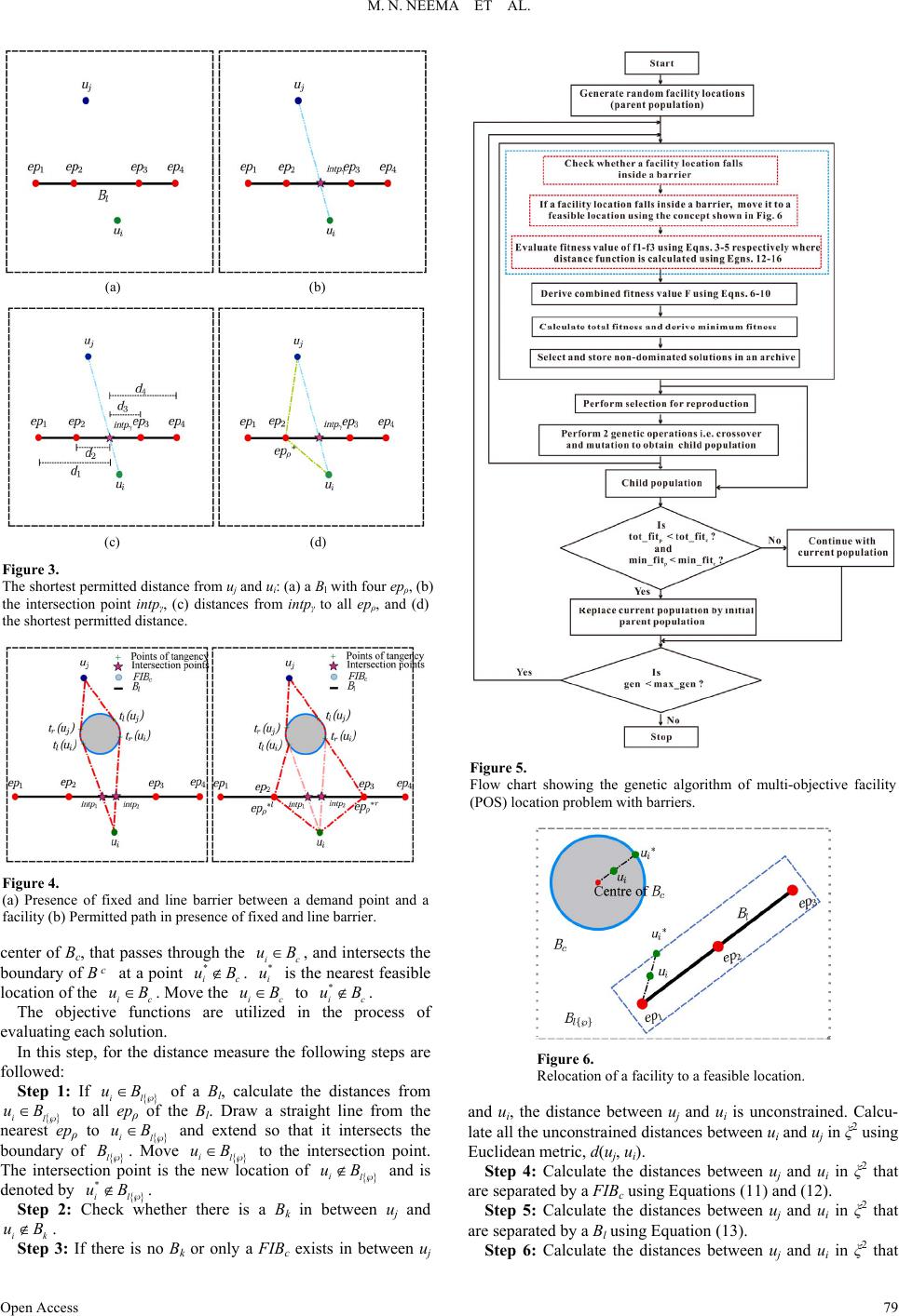

M. N. NEEMA ET AL.

(a) (b)

Figure 3.

The shortest permitted distance from uj and ui: (a) a Bl with four epρ, (b)

the intersection point intpγ, (c) distances from intpγ to all epρ, and (d)

the shortest permitted distance.

Figure 4.

(a) Presence of fixed and line barrier between a demand point and a

facility (b) Permitted path in presence of fixed and line barrier.

center of Bc, that passes through the c

, and intersects the

boundary of Bc at a point . is the nearest feasible

location of the . Move the to .

uB

uB

ic ic

The objective functions are utilized in the process of

evaluating each solution.

uB*

uB

In this step, for the distance measure the following steps are

followed:

Step 1: If





 of a Bl, calculate the distances from





 to all epρ of the Bl. Draw a straight line from the

nearest epρ to





 and extend so that it intersects the

boundary of





. Move





 to the intersection point.

The intersection point is the new location of





 and is

denoted by .



Step 2: Check whether there is a Bk in between uj and





uBk

Step 3: If there is no Bk or only a FIBc exists in between uj

Figure 5.

Flow chart showing the genetic algorithm of multi-objective facility

(POS) location problem with barri ers.

Figure 6.

Relocation of a facility to a feasible location.

and ui, the distance between uj and ui is unconstrained. Calcu-

late all the unconstrained distances between ui and uj in ξ2 using

Euclidean metric, d(uj, ui).

Step 4: Calculate the distances between uj and ui in ξ2 that

are se parated by a FIBc using Equations (11) and (12).

Step 5: Calculate the distances between uj and ui in ξ2 that

are se parated by a Bl using Equation (13).

Step 6: Calculate the distances between uj and ui in ξ2 that

Open Access 79

M. N. NEEMA ET AL.

are separated by both of FIBc and Bl using Equations (14) and

(15).

The non-dominated solutions are sorted from the obtained

solutions to store it in an archive. The selection process for re-

production saves the better solutions. Therefore, the stronger

(having better fitness) chromosomes survive, while weaker

chromosomes die out. We follow roulette wheel selection me-

thod. For the reproduction process, genetic operations are per-

formed in the parent chromosomes. This will generate off-

spring chromosomes. In our GA, a single-point crossover op-

eration is carried out, where two parent chromosomes inter-

change their genetic material (bits) after a randomly decided

single point. The mutation operation is performed to bring di-

versity of the solutions in the offspring population. Mutation is

a random change of one or more bits. In the reproduction proc-

ess to perform the next generation, we choose the better one

between the parent and the offspring population. The total fit-

ness and the minimum fitness of both population are com-

pared for this selection.

Figure 5 shows the GA process used for multi-objective

POS location problem with barriers. The GA process continues

until the prefixed number of generations has bee n reached. After

finishing the GA cycle, final sorting of non-dominated solu-

tions is performed among the solutions stored in the archive.

Next, we present a case study applying the multi-objective

model with barriers to find the approximate optimal locations

of some new POS in Dhaka city.

A Case Study on Dhaka City

In our previous research, we showed 0.22 acres per 1000

people open space is available in Dhaka city. This is far below

the recommended standards in different countries in the world

(Neema & Ohgai, 2010). As noted parks and green areas in

Dhaka city have been diminished significantly during the last

four decades. The continuous growth of population is presume-

bly the underlying mainstay of such depletion. In contrary, a

well distributed optimized green space is regarded as one of the

main ingredients of an environmentally friendly city. The opti-

mal locations were obtained simultaneously optimizing three

multiple objectives i.e. POS near: a) populated areas, b) air

quality degraded area, and c) noise pollution areas including a

constraint (barrier).

The prime objective of this case study is to locate some new

parks and open spaces in Dhaka city. For modelling purpose,

we assume there are some demand generating points in the

problem space Dhaka. The centroids of city wards (a total of 90

wards) are considered as the demand points whose spatial coor-

dinates and demands are known. As the model is formulated

with continuous optimization scheme, any place could be a po-

tential site for a POS. But the problem is that there are various

constraints in reality especially many existing barriers of dif-

ferent types and sizes. Therefore, we need to incorporate these

barrier constraints into the model to avoid unrealistic POS

planning in any of such barriers. The required input data for the

model was prepared employing ArcGIS 9.1 software. The fol-

lowing procedures and consideration were adopted:

1) We confined the problem space with the bounding rectan-

gle of the city.

2) The centroids of 90 wards of the city is considered as the

demand generating points. Three levels of demand (i.e. popula-

tion, air quality, noise level) of each ward are assigned as the

weights to each demand point. Details can be found elsewhere

(Neema & Ohgai, 2010).

3) We consider the existing parks and open space, industrial

areas and market areas of the city as fixed barriers FIBc, the

water bodies of the city as flexible barriers FLBc and the lakes

of the city as line barriers Bl. The total number of FIBc, FIBc

and Bl are respectively 219, 119 and 6. We exclude the rivers

from our barrier considerations as it passes mostly through the

outside of the ward areas. To simply the model, we merge some

small existing barriers.

4) We set the numbers of new POS in the problem space to

be 30, each of which contains 50 acres of area. Details of these

considerations can be found in ((Neema & Ohgai, 2010) where

we estimated that the city needs 1505 acres of area for

additional POS. For the sake of simplification of simulation, we

assume the size of all new POS is to be equal.

Now, we represent the spatial distribution of existing barriers

and different levels of demand for providing more POS. It can

be observed that there exist different types and sizes of physical

barriers in Dhaka, shown in Figure 7(a). There are a big Indus-

trial region, some existing POS and a lake in the central part, a

large existing POS in the northern part, some small industrial

regions in the southern part, some lakes in the eastern part, and

market areas and small size water bodies throughout the city.

Among these barrier regions, we represent the elongated shaped

barriers using line shapes Bl whose exit points are denoted by

epρ and non-elongated shapes using circular shapes Bc. We

included the barriers in the coding of the model to restrict plac-

ing new POS locations within these regions.

The calculated ward-wise population distribution (required

for objective function f1) is presented in Figure 7(b). Specifi-

cally many highly populated areas are devoid of sufficient

numbers of POS. POSs are mostly concentrated in a few places

and extensive areas are lack of it.

Depicted in Figure 7(c) is the ward-wise air quality distribu-

tion (required for objective function f2) in the city. For ai r qual-

ity data we considered the concentration of SO2 in the air. An

area is considered to be polluted when the average SO2 concen-

tration is above 40 ppb level.

Evidently, there are significant spatial variations and ex-

tremely high concentrations of SO2 in the central and the south-

eastern industrial-zone of the city. The maximum level of SO2

is 100 ppb which also agrees well with a previous report (Azad

& Kitada, 1998). Reportedly, the air-pollution enclaves north-

west to south-east regions including the regions that fall along-

side the river (Buriganga).

Basically, Dhaka being the capital city and the hub of com-

mercial activity, the air-pollution problem of it is more acute.

The air quality of the city is being badly degraded day by day.

Noise level distribution (required for objective function f3) of

the city is presented in Figure 7(d). As expected, the areas of

the city with existing POS and lakes have less noise pollution.

It reveals that POS and lakes do have a significant impact on

reducing noise level. So, noise level is considered as another

objective function in the model to reduce noise level of the city

by providing more POS (i.e. green areas) near noise polluted

areas.

Next, we present modeling results to show the effective im-

plementation of the multi-objective model with barriers.

Results

The genetic algorithm (GA) of the model was coded in C++

Open Access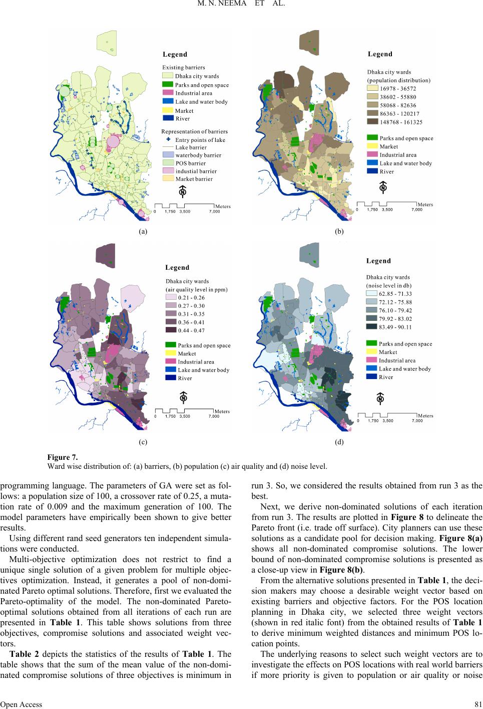

M. N. NEEMA ET AL.

Open Access 81

(a) (b)

Figure 7.

Ward wise distribution of: (a) barriers, (b) population (c) air quality and (d) noise level.

programming language. The parameters of GA were set as fol-

lows: a population size of 100, a crossover rate of 0.25, a muta-

tion rate of 0.009 and the maximum generation of 100. The

model parameters have empirically been shown to give better

results.

Using different rand seed generators ten independent simula-

tions were conducted.

Multi-objective optimization does not restrict to find a

unique single solution of a given problem for multiple objec-

tives optimization. Instead, it generates a pool of non-domi-

nated Pareto optimal solutions. Therefore, first we evaluated the

Pareto-optimality of the model. The non-dominated Pareto-

optimal solutions obtained from all iterations of each run are

presented in Table 1. This table shows solutions from three

objectives, compromise solutions and associated weight vec-

tors.

Table 2 depicts the statistics of the results of Table 1. The

table shows that the sum of the mean value of the non-domi-

nated compromise solutions of three objectives is minimum in

run 3. So, we considered the results obtained from run 3 as the

best.

Next, we derive non-dominated solutions of each iteration

from run 3. The results are plotted in Figure 8 to delineate the

Pareto front (i.e. trade off surface). City planners can use these

solutions as a candidate pool for decision making. Figure 8(a)

shows all non-dominated compromise solutions. The lower

bound of non-dominated compromise solutions is presented as

a close-up view in Figure 8(b).

From the alternative solutions presented in Table 1, the deci-

sion makers may choose a desirable weight vector based on

existing barriers and objective factors. For the POS location

planning in Dhaka city, we selected three weight vectors

(shown in red italic font) from the obtained results of Table 1

to derive minimum weighted distances and minimum POS lo-

cation points.

The underlying reasons to select such weight vectors are to

investigate the effects on POS locations with real world barriers

if more priority is given to population or air quality or noise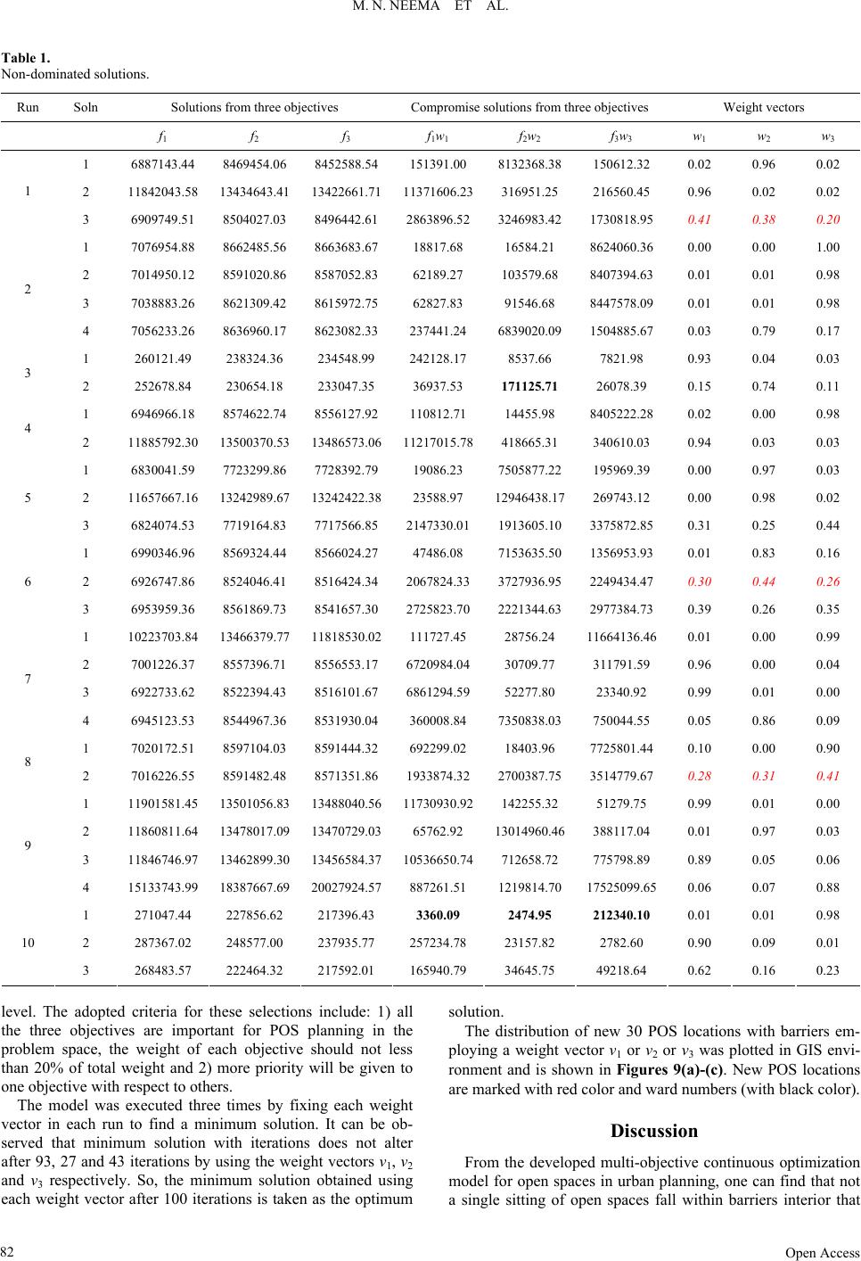

M. N. NEEMA ET AL.

Table 1.

Non-dominated solutions.

Run Soln Solution s from three objectives Compromise solutions from three objectives Weight vectors

f1 f2 f3 f1w1 f2w2 f3w3 w1 w2 w3

1 6887143.44 8469454.06 8452588.54 151391.00 8132368.38 150612.32 0.02 0.96 0.02

2 11842043.58 13434643.41 13422661.7111371606.23316951.25 216560.45 0.96 0.02 0.02

3 6909749.51 8504027.03 8496442.61 2863896.52 3246983.42 1730818.95 0.41 0.38 0.20

1 7076954.88 8662485.56 8663683.67 18817.68 16584.21 8624060.36 0.00 0.00 1.00

2 7014950.12 8591020.86 8587052.83 62189.27 103579.68 8407394.63 0.01 0.01 0.98

3 7038883.26 8621309.42 8615972.75 62827.83 91546.68 8447578.09 0.01 0.01 0.98

4 7056233.26 8636960.17 8623082.33 237441.24 6839020.09 1504885.67 0.03 0.79 0.17

1 260121.49 238324.36 234548.99 242128.17 8537.66 7821.98 0.93 0.04 0.03

3 2 252678.84 230654.18 233047.35 36937.53 171125.71 26078.39 0.15 0.74 0.11

1 6946966.18 8574622.74 8556127.92 110812.71 14455.98 8405222.28 0.02 0.00 0.98

4 2 11885792.30 13500370.53 13486573.0611217015.78418665.31 340610.03 0.94 0.03 0.03

1 6830041.59 7723299.86 7728392.79 19086.23 7505877.22 195969.39 0.00 0.97 0.03

2 11657667.16 13242989.67 13242422.3823588.97 12946438.17269743.12 0.00 0.98 0.02 5

3 6824074.53 7719164.83 7717566.85 2147330.01 1913605.10 3375872.85 0.31 0.25 0.44

1 6990346.96 8569324.44 8566024.27 47486.08 7153635.50 1356953.93 0.01 0.83 0.16

2 6926747.86 8524046.41 8516424.34 2067824.33 3727936.95 2249434.47 0.30 0.44 0.26 6

3 6953959.36 8561869.73 8541657.30 2725823.70 2221344.63 2977384.73 0.39 0.26 0.35

1 10223703.84 13466379.77 11818530.02111727.45 28756.24 11664136.46 0.01 0.00 0.99

2 7001226.37 8557396.71 8556553.17 6720984.04 30709.77 311791.59 0.96 0.00 0.04

3 6922733.62 8522394.43 8516101.67 6861294.59 52277.80 23340.92 0.99 0.01 0.00

4 6945123.53 8544967.36 8531930.04 360008.84 7350838.03 750044.55 0.05 0.86 0.09

1 7020172.51 8597104.03 8591444.32 692299.02 18403.96 7725801.44 0.10 0.00 0.90

8 2 7016226.55 8591482.48 8571351.86 1933874.32 2700387.75 3514779.67 0.28 0.31 0.41

1 11901581.45 13501056.83 13488040.5611730930.92142255.32 51279.75 0.99 0.01 0.00

2 11860811.64 13478017.09 13470729.0365762.92 13014960.46388117.04 0.01 0.97 0.03

3 11846746.97 13462899.30 13456584.3710536650.74712658.72 775798.89 0.89 0.05 0.06

4 15133743.99 18387667.69 20027924.57887261.51 1219814.70 17525099.65 0.06 0.07 0.88

1 271047.44 227856.62 217396.43 3360.09 2474.95 212340.10 0.01 0.01 0.98

2 287367.02 248577.00 237935.77 257234.78 23157.82 2782.60 0.90 0.09 0.01 10

3 268483.57 222464.32 217592.01 165940.79 34645.75 49218.64 0.62 0.16 0.23

level. The adopted criteria for these selections include: 1) all

the three objectives are important for POS planning in the

problem space, the weight of each objective should not less

than 20% of total weight and 2) more priority will be given to

one objective with respect to others.

The model was executed three times by fixing each weight

vector in each run to find a minimum solution. It can be ob-

served that minimum solution with iterations does not alter

after 93, 27 and 43 iterations by using the weight vectors v1, v2

and v3 respectively. So, the minimum solution obtained using

each weight vector after 100 iterations is taken as the optimum

solution.

The distribution of new 30 POS locations with barriers em-

ploying a weight vector v1 or v2 or v3 was plotted in GIS envi-

ronment and is shown in Figures 9(a)-(c). New POS locations

are marked with red color and ward numbers (with black color).

Discussion

From the developed multi-objective continuous optimization

model for open spaces in urban planning, one can find that not

a single sitting of open spaces fall within barriers interior that

Open Access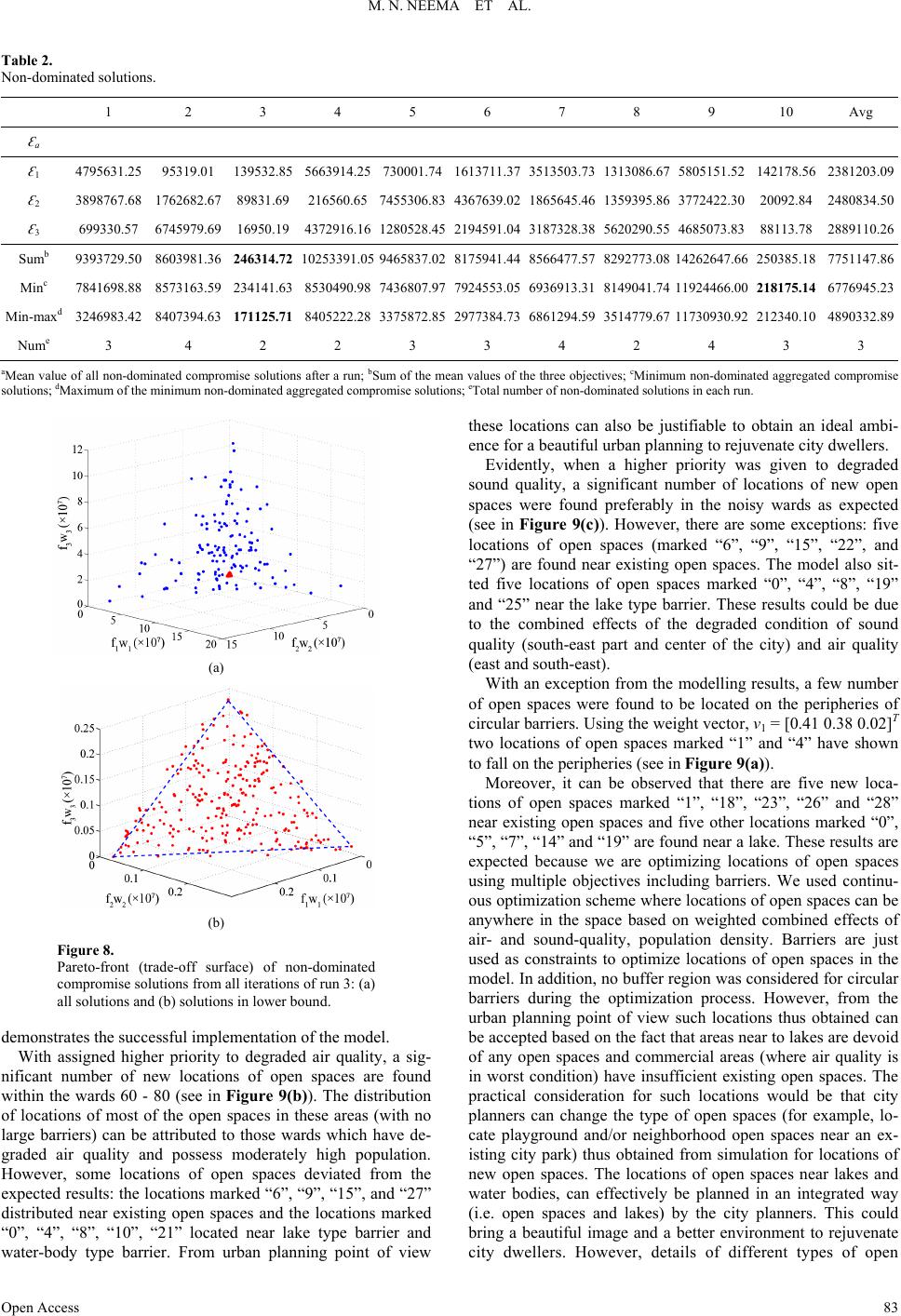

M. N. NEEMA ET AL.

Table 2.

Non-dominated solutions.

1 2 3 4 5 6 7 8 9 10 Avg

Ɛa

Ɛ1 4795631.25 95319.01 139532.85 5663914.25730001.741613711.373513503.731313086.675805151.52 142178.562381203.09

Ɛ2 3898767.68 1762682.6789831.69 216560.657455306.834367639.021865645.461359395.863772422.30 20092.842480834.50

Ɛ3 699330.57 6745979.6916950.19 4372916.161280528.452194591.043187328.385620290.554685073.83 88113.782889110.26

Sumb 9393729.50 8603981.36246314.72 10253391.05 9465837.028175941.448566477.578292773.08 14262647.66 250385.187751147.86

Minc 7841698.88 8573163.59234141.63 8530490.987436807.977924553.056936913.318149041.7411924466.00

218175.14 6776945.23

Min-maxd 3246983.42 8407394.63171125.71 8405222.283375872.852977384.736861294.593514779.67 11730930.92 212340.104890332.89

Nume 3 4 2 2 3 3 4 2 4 3 3

aMean value of all non-domina ted compromise solutions afte r a run; bSum of the mean values of the three objectives; cMinimum non-dominated aggregated compromise

solutions; dMaximum of the minimum non-dominated aggregated compromise solutions; eTot al number of non-dominated s olutions in each run.

(a)

(b)

Figure 8.

Pareto-front (trade-off surface) of non-dominated

compromise solutions from all iterations of run 3: (a)

all solutions and (b) so l u ti o n s i n l o we r bound.

demonstrates the successful implementation of the model.

With assigned higher priority to degraded air quality, a sig-

nificant number of new locations of open spaces are found

within the wards 60 - 80 (see in Figure 9(b)). The distribution

of locations of most of the open spaces in these areas (with no

large barriers) can be attributed to those wards which have de-

graded air quality and possess moderately high population.

However, some locations of open spaces deviated from the

expected results: t he locations marked “6”, “9”, “15”, and “27”

distributed near existing open spaces and the locations marked

“0”, “4”, “8”, “10”, “21” located near lake type barrier and

water-body type barrier. From urban planning point of view

these locations can also be justifiable to obtain an ideal ambi-

ence for a beautiful urban planning to rejuvenate city dwellers.

Evidently, when a higher priority was given to degraded

sound quality, a significant number of locations of new open

spaces were found preferably in the noisy wards as expected

(see in Figure 9(c)). However, there are some exceptions: five

locations of open spaces (marked “6”, “9”, “15”, “22”, and

“27”) are found near existing open spaces. The model also sit-

ted five locations of open spaces marked “0”, “4”, “8”, “19”

and “25” near the lake type barrier. These results could be due

to the combined effects of the degraded condition of sound

quality (south-east part and center of the city) and air quality

(east and south-east).

With an exception from the modelling results, a few number

of open spaces were found to be located on the peripheries of

circular barriers. Using the weight vector, v1 = [0.41 0.38 0.02]T

two locations of open spaces marked “1” and “4” have shown

to fall on the peripheries (see in Figure 9(a)).

Moreover, it can be observed that there are five new loca-

tions of open spaces marked “1”, “18”, “23”, “26” and “28”

near existing open spaces and five other locations marked “0”,

“5”, “7”, “14” and “19” are found near a lake. These results are

expected because we are optimizing locations of open spaces

using multiple objectives including barriers. We used continu-

ous optimization scheme where locations of open spaces can be

anywhere in the space based on weighted combined effects of

air- and sound-quality, population density. Barriers are just

used as constraints to optimize locations of open spaces in the

model. In addition, no buffer region was considered for circular

barriers during the optimization process. However, from the

urban planning point of view such locations thus obtained can

be accepted based on the fact that areas near to lakes are devoid

of any open spaces and commercial areas (where air quality is

in worst condition) have insufficient existing open spaces. The

practical consideration for such locations would be that city

planners can change the type of open spaces (for example, lo-

cate playground and/or neighborhood open spaces near an ex-

isting city park) thus obtained from simulation for locations of

new open spaces. The locations of open spaces near lakes and

water bodies, can effectively be planned in an integrated way

(i.e. open spaces and lakes) by the city planners. This could

bring a beautiful image and a better environment to rejuvenate

city dwellers. However, details of different types of open

Open Access 83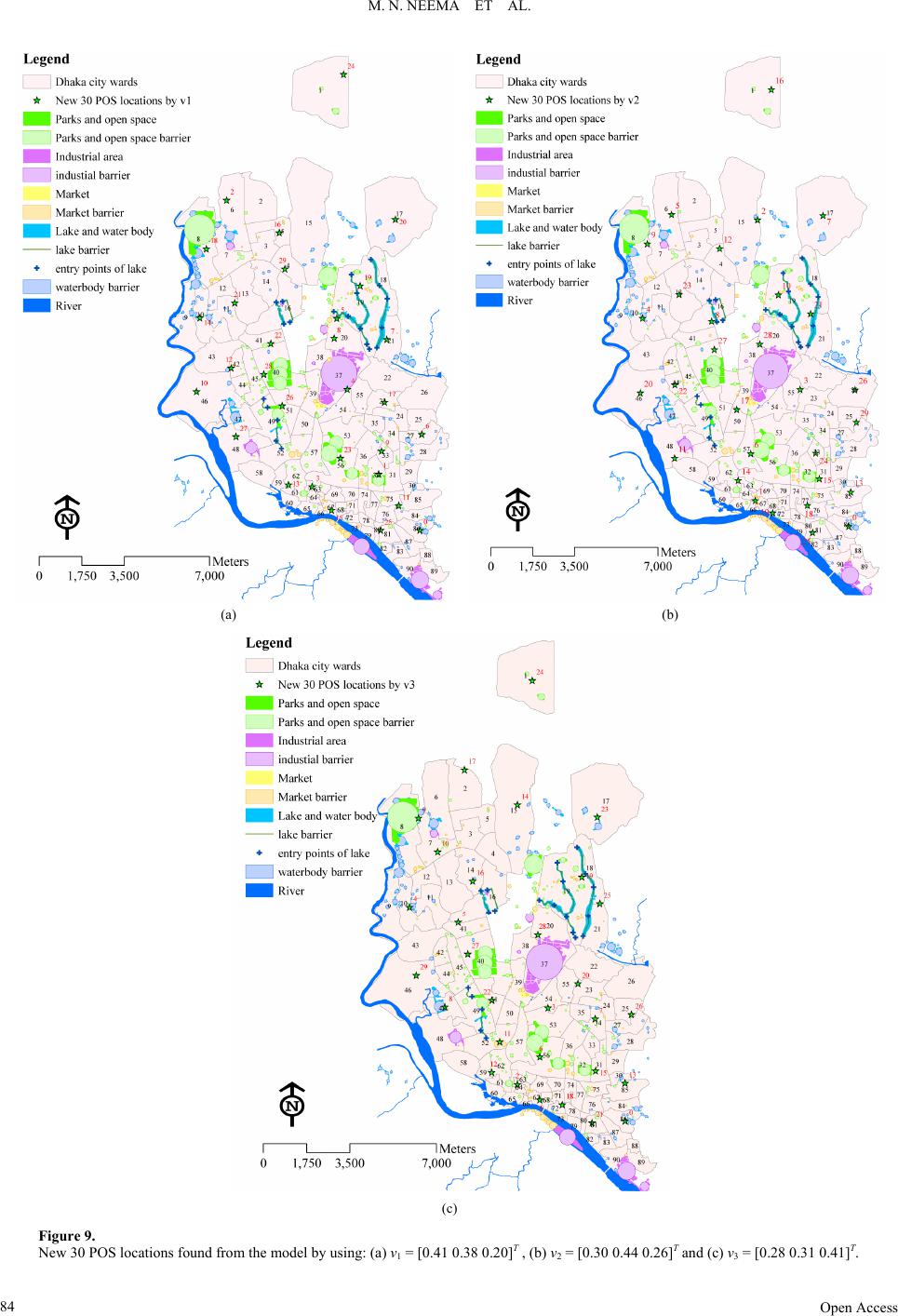

M. N. NEEMA ET AL.

(a) (b)

(c)

Figure 9.

New 30 POS locations found from the model by using: (a) v1 = [0.41 0.38 0.20]T , (b) v2 = [0.30 0.44 0.26]T and (c) v3 = [0.28 0.31 0.41]T.

Open Access

M. N. NEEMA ET AL.

spaces are beyond the scope of this paper.

However, to prevent the sitting (from simulations) of some

new open spaces on the peripheries of barriers a pre-determined

buffer region can be used. Indeed, considering a buffer zone

from line barriers, the model has shown well distribution of

open spaces exterior to the existing lake type barriers. For in-

stance, locations of open spaces marked “5”, “7” and “19” in

Figure 9(a), location marked “21” in Figure 9(b) and location

marked “9” in Figure 9(c) are completely outside to the pe-

ripheries of lake type barriers.

Conclusion

In this research, we developed an intelligent multi-objective

continuous optimization model with a new approach for green

urbanism in a city. This modelling approach seeks the optimum

places for providing new parks and open spaces for greeneries

throughout a city. Application of the model in Dhaka city has

successfully demonstrated to provide optimal locations of addi-

tional POS. Adequate numbers of POS were found in environ-

mentally degraded areas with air and noise pollution. In addi-

tion, the obtained locations of open spaces found near lakes and

water bodies have shown to be planned in an integrated way (i.e.

open spaces and lakes) by the city planners to bring a beautiful

image and a better environment to rejuvenate city dwellers. As

the developed powerful continuous optimization scheme in

GA-based multi-objective model searches for a pool of non-

dominated Pareto optimal solutions, city planners can choose

an alternative solution which is best suited for the prevailing

land-use pattern in a city (if it is necessary by averting locations

from city centre and developed residential areas choosing an

appropriate solution from the pool). This model could equally

be applicable in any city for providing optimum locations of

POS. Following our approach, a well-planned urban greening

can thus be realized to maintain a healthy sustainable city.

However, the scope of the present study is currently limited to

site the optimal locations of POS (especially for the purpose of

urban greeneries), in future study it would be an interesting

research aspect to incorporate wetlands and water bodies to find

out optimum locations for all eco logical reserves.

Acknowledgements

This research was conducted under Japanese Government

Scholarship funding. We also acknowledge the funding from

Hori Information Science Promotion Foundation, Japan.

REFERENCES

Azad, A., & Kitada, T. (1998). Characteristics of the air pollution in the

city of dhaka, bangladesh in winter. Atmospheric Environment, 32,

1991-2005. http://dx.doi.org/10.1016/S1352-2310(97)00508-6

BenDor, T., Westervelt, J., Song, Y., & Sexton, J. (2013). Modeling

park development through regional land use change simulation. Land

Use Policy, 30, 1-12.

http://dx.doi.org/10.1016/j.landusepol.2012.01.012

Borrego, C., Martins, H., Tchepel, O., Salmim, L., Monteiro, A., &

Miranda, A. I. (2006). How urban structure can affect city sustain-

ability from an air quality perspective. Environmental Modelling &

Software, 21, 461- 467.

http://dx.doi.org/10.1016/j.envsoft.2004.07.009

Camm, J., Norman, S., Polasky, S., & Solow, A. (2002). Nature reserve

site selection to maximize expected species covered. Operations Re-

search, 50, 946-955.

Chiesura, A. (2004). The role of urban parks for the sustainable city.

Landscape Urban Plan, 68, 129-138.

http://dx.doi.org/10.1016/j.landurbplan.2003.08.003

Choumert, J. (2010). An empirical investigation of public choices for

green spaces. Land Use Policy, 27, 1123-1131.

Drechsler, M., & Wätzold, F. (2001). The importance of economic cost

in the development of guidelines for spatial conservation manage-

ment. Biological Conservation, 97, 51-59.

http://dx.doi.org/10.1016/S0006-3207(00)00099-9

Egger, S. (2006). Determining a sustainable city model. Environmental

Modelling & Software, 21, 1235-1246.

http://dx.doi.org/10.1016/j.envsoft.2005.04.012

Fonseca, C. M., & Fleming, P. J. (1991). An overview of evolutionary

algorithms in multiobjective optimization. Evolutionary Computation,

3, 1-16. http://dx.doi.org/10.1162/evco.1995.3.1.1

Gobster, P. H. (1998). Urban parks as green walls or green magnets?

interracial relations in neighborhood boundary parks. Landscape

Urban Plan, 41, 43-55.

http://dx.doi.org/10.1016/S0169-2046(98)00045-0

Katz, N., & Cooper, L. (1981). Facility location in the presence of

forbidden regions, i: Formulation and the case of euclidean distance

with one forbidden circle. European Journal of Operational Re-

search, 6, 166-173. http://dx.doi.org/10.1016/0377-2217(81)90203-4

Klamroth, K. (2004). Algebraic properties of location problems with

one circular barrier. European Journal of Operational Research, 154,

20-35. http://dx.doi.org/10.1016/0377-2217(81)90203-4

Kong, F., Yinb, H., Nakagoshic, N., & Zongb, Y. (2010). Urban green

space network development for biodiversity conservation: Identifica-

tion based on graph theory and gravity modeling. Landscape Urban

Plan, 95, 16-27. http://dx.doi.org/10.1016/j.landurbplan.2009.11.001

Lam, K. C., Ng, S. L., Hui, W. C., & Chan, P. K. (2005). Environ-

mental quality of urban parks and open spaces in Hong Kong. Envi-

ronmental Monitoring and Assessment, 111, 55-73.

http://dx.doi.org/10.1007/s10661-005-8039-2

McDonnell, M., Possingham, H., Ball, I., & Cousins, E. (2002). Math-

ematical methods for spatially cohesive reserve design. Journal of

Environmental Modeling and Assessment, 7, 107-114.

Morancho, A. B. (2003). A hedonic valuation of urban green areas.

Landscape Urban Plan, 66, 35-41.

http://dx.doi.org/10.1016/S0169-2046(03)00093-8

Neema, M.N., Ohgai, A., & Emanuel, L. (2008). Analyzing existing

condition and location of open spaces in Dhaka city. Proceedings of

6th Int. Symposium on City Planning and Urban Management in

Asian Countries, Jinju.

Neema, M. N., & Ohgai, A. (2010). Multi-objective location modeling

of urban parks and open space s: Continuous optimization. Computers,

Environment and Urban Systems, 34, 359-376.

http://dx.doi.org/10.1016/j.compenvurbsys.2010.03.001

Neema, M. N., Maniruzzaman, K. M., & Ohgai, A. (2011). New ge-

netic algorithms based approaches to continuous p-median problem.

Networks and Spatial Economics, 11, 83- 99.

http://dx.doi.org/10.1007/s11067-008-9084-5

Neema, M.N., Maniruzzaman, K. M., & Ohgai, A. (2013). Green ur-

banism incorporating greenery-based conceptual model towards at-

taining a sustainable healthy livable environment—Dhaka City’s

perspective. Current Urban Studies, 1, 19-27.

http://dx.doi.org/10.4236/cus.2013.13003

Neema, M.N., & Ohgai, A. (2013). Multitype green-space modeling for

urban planning using GA and GIS. Environment and Planning B:

Planning and Design, 40, 447-473. http://dx.doi.org/10.1068/b38003

Nordh, H., Hartigb, T., Hagerhalla, C., & Frya, G. (2009). Components

of small urban parks that predict the possibility for restoration. Ur-

ban Forestry Urban Greening, 8, 225-235.

http://dx.doi.org/10.1016/j.ufug.2009.06.003

Poggio, L., & Vräcaj, B. (2009). A GIS-based human health risk as-

sessment for urban green space planning-an example from grugliasco

(Italy). Science of the Total Environment, 407, 5961-5970.

http://dx.doi.org/10.1016/j.scitotenv.2009.08.026

Schipperijn, J., Stigsdotter, U., Randrup, T. B., & Troelsen, J. (2010).

Influences on the use of urban green space-a case study in odense,

denmark. Urban Forestry & Urban Greening, 9, 25-32.

http://dx.doi.org/10.1016/j.ufug.2009.09.002

Sdnp, B. (2005). Green Cities Plan for the Planet (Digital Publication).

Open Access 85

M. N. NEEMA ET AL.

Dhaka: World Enviornm e n t D ay.

Szeremeta, B., Henrique, P., & Zannin, T. (2009). Analysis and evalua-

tion of soundscapes in public parks through interviews and meas-

urement of noise. Science of the Total Environment, 407, 6143-6149.

http://dx.doi.org/10.1016/j.scitotenv.2009.08.039

Uddin, N. (2005). The relationship between Urban Forestry and Pov-

erty Alleviation-Dhaka as a case study. Master Degree Project, Al-

narp: Swedish University of Agricultural Sciences ,.

Uy, P., & Nakagoshi, N. (2008). Application of land suitability analysis

and landscape ecology to urban green space planning in Hanoi,

Vietnam. Urban Forestry Urban Greening, 7, 25-40.

http://dx.doi.org/10.1016/j.ufug.2007.09.002

Zhang, X., & Armstrong, M. P. (2008). Genetic algorithms and the

corridor location problem: multiple objectives and alternative solu-

tions. Environment and Planning B, 35, 148-168.

http://dx.doi.org/10.1068/b32167

Open Access
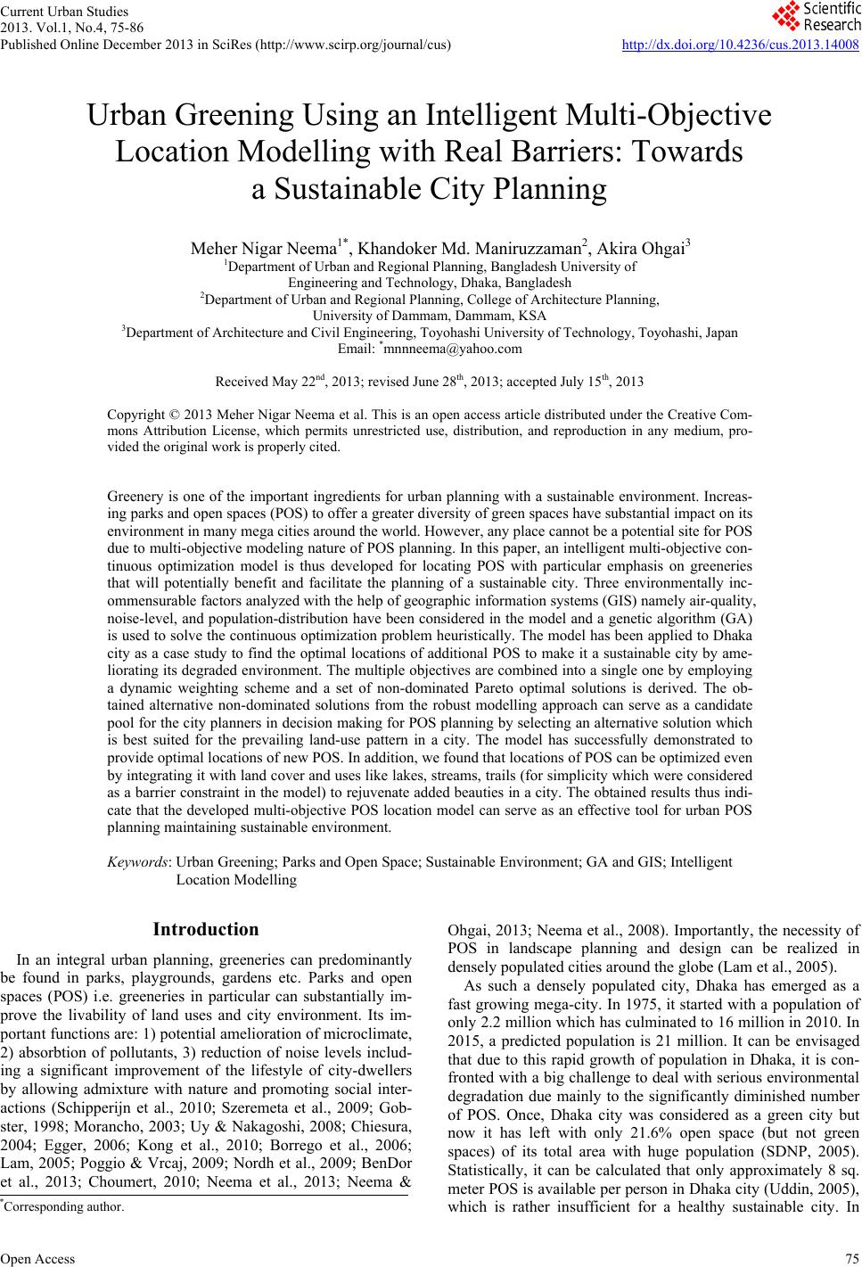