 Low Carbon Economy, 2013, 4, 24-34 Published Online December 2013 (http://www.scirp.org/journal/lce) http://dx.doi.org/10.4236/lce.2013.44A003 Open Access LCE Development of an Agent-Based Model and Its Application to the Estimation of Global Carbon Emiss ions Paula Castesana1, Salvador Puliafito2 1Facultad Regional Buenos Aires, Universidad Tecnológica Nacional, Buenos Aires, Argentina; 2CONICET-Universidad Tec- nológica Nacional, Mendoza, Argentina. Email: pcastesana@gmail.com, enrique_puliafito@yahoo.com.ar Received October 23rd, 2013; revised November 17th, 2013; accepted November 24th, 2013 Copyright © 2013 Paula Castesana, Salvador Puliafito. This is an open access article distributed under the Creative Commons Attri- bution License, which permits unrestricted use, distribution, and reproduction in any medium, provided the original work is properly cited. ABSTRACT With the purpose of studying the influence of population dynamics and economic growth on energy consumption and carbon emissions, an endogenous economic growth model is proposed incorporating physical and human capital and using an Agent-Based Model. The model can test different development strategies by identifying the key factors exist- ing at the agent level that may speed up or slow down a given path, an d therefore it is an interesting tool to develop and to test mitigation and/or adaptation measures. Favorable scenarios may be possible in societies that encourage invest- ment in human capital through edu cation and technolog ical development, provided th at this is accompanied by a reduc- tion in consumption rates and the creation of physical capital by the population. Moreover, this model shows that hu- man capital resulting from education not only raises productivity, but also plays a key role in the development and adoption of new technologies th at drive long-term growth. Keywords: Agent-Based Modeling; Carbon Emissions; Economic Growth; Energy Consumption; Population Dynamics 1. Introduction The ri se of the a tmosph eric carbon dioxid e concen tration due to anthropogenic emissions generated by energy con- sumption of fossil fuels is increasing the additional greenhouse effect. Currently, the analysis of the influen ce of demographic variables on these emissions has be- come a relevant subject in the debate on climate change, since their impact on economic growth has a direct effect on the consu mption of goods, primary energy, and there- fore on carbon emissions, modifying the accumulation of greenhouse gases in the atmosphere. Population growth rates have declined over the last fifty years in almost every country in the world, showing a reduction in fertility rates and an increase in life exp ec- tancy at birth [1]. The significant social and health care improvement of the last century has decreased infant mortality and increased longevity, producing a demogra- phic transition which has changed the population struc- ture. In developed countries, a reduction of the youngest age groups is already noticeable, however smoothed by immigration from less developed countries. Global popu- lation ageing may impact on economic growth through variations in consumptions preferences. Theories of economic growth have led to the devel- opment of many studies since the beginning of the sys- tematization of this science. Among such theories, we can mention Adam Smith, who proposed the division of labor as a source of growth. Thomas Malthus stated that if income exceeds a certain threshold, mortality rates should decay and birth rates should rise, balancing eco- nomic growth. However, data of the past 150 years show that while mortality rates declined due to improved liv ing conditions and investment in health, birth rates also de- creased in most countries. Neoclassical economists have suggested that the causes of economic growth are related to increased investment in physical capital through an exogenous technical progress, ignoring its relationship with population dynamics [2,3]. But increased invest- ment does not adequately explain the decline in growth rates or the difference in growth between developed and least developed countries. Endogenous growth models determine long-term 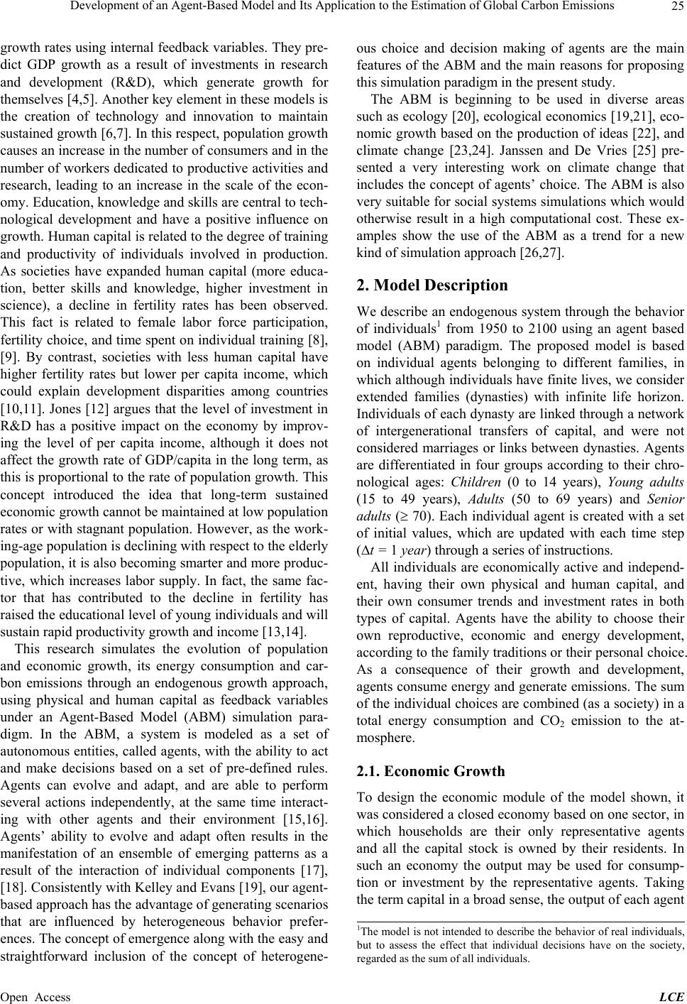 Development of an Agent-Based Model and Its Application to the Estimation of Global Carbon Emissions 25 growth rates using internal feedback variables. They pre- dict GDP growth as a result of investments in research and development (R&D), which generate growth for themselves [4,5]. Another key element in these models is the creation of technology and innovation to maintain sustained growth [6,7]. In this respect, population growth causes an increase in the number of consumers and in the number of workers dedicated to produ ctive activities and research, leading to an increase in the scale of the econ- omy. Education, knowledge an d skills are central to tech- nological development and have a positive influence on growth. Human capital is related to the degree of training and productivity of individuals involved in production. As societies have expanded human capital (more educa- tion, better skills and knowledge, higher investment in science), a decline in fertility rates has been observed. This fact is related to female labor force participation, fertility choice, and time spent on individu al training [8], [9]. By contrast, societies with less human capital have higher fertility rates but lower per capita income, which could explain development disparities among countries [10,11]. Jones [12] argues that the level of investment in R&D has a positive impact on the economy by improv- ing the level of per capita income, although it does not affect the growth rate of GDP/capita in the long term, as this is proportional to the rate of population growth. Th is concept introduced the idea that long-term sustained economic growth cannot be maintained at low populatio n rates or with stagnant population. However, as the work- ing-age popu lation is declining with respect to the elderly population, it is also becoming smarter and more produc- tive, which increases labor supply. In fact, the same fac- tor that has contributed to the decline in fertility has raised the educational level of yo ung individuals and will sustain rapid productivity growth and inco me [13,14]. This research simulates the evolution of population and economic growth, its energy consumption and car- bon emissions through an endogenous growth approach, using physical and human capital as feedback variables under an Agent-Based Model (ABM) simulation para- digm. In the ABM, a system is modeled as a set of autonomous entities, called agents, with the ability to act and make decisions based on a set of pre-defined rules. Agents can evolve and adapt, and are able to perform several actions independently, at the same time interact- ing with other agents and their environment [15,16]. Agents’ ability to evolve and adapt often results in the manifestation of an ensemble of emerging patterns as a result of the interaction of individual components [17], [18]. Consistently with Kelley and Ev ans [19], our agen t- based approach has the advantage of generating scenarios that are influenced by heterogeneous behavior prefer- ences. The concept of emergence along with the easy and straightforward inclusion of the concept of heterogene- ous choice and decision making of agents are the main features of the ABM and the main reasons for proposing this simulation paradigm in the present study. The ABM is beginning to be used in diverse areas such as ecology [20], eco logical economics [19,21], eco- nomic growth based on the production of ideas [22], and climate change [23,24]. Janssen and De Vries [25] pre- sented a very interesting work on climate change that includes the concept of agents’ choice. The ABM is also very suitable for social systems simulations which would otherwise result in a high computational cost. These ex- amples show the use of the ABM as a trend for a new kind of simulation approach [26,27]. 2. Model Description We describe an endogenous system through the behavior of individuals1 from 1950 to 2100 using an agent based model (ABM) paradigm. The proposed model is based on individual agents belonging to different families, in which although ind ividuals have finite lives, we cons ider extended families (dynasties) with infinite life horizon. Individuals of each dynasty are linked through a network of intergenerational transfers of capital, and were not considered marriages or links between dynasties. Agents are differentiated in four groups according to their chro- nological ages: Children (0 to 14 years), Young adults (15 to 49 years), Adults (50 to 69 years) and Senior adults ( 70). Each individual agent is created with a set of initial values, which are updated with each time step (t = 1 year) through a series of instructions. All individuals are economically active and independ- ent, having their own physical and human capital, and their own consumer trends and investment rates in both types of capital. Agents have the ability to choose their own reproductive, economic and energy development, according to the family traditions or their personal choice. As a consequence of their growth and development, agents consume energy and generate emissions. The sum of the individual choices are combined (as a society) in a total energy consumption and CO2 emission to the at- mosphere. 2.1. Economic Growth To design the economic module of the model shown, it was considered a closed economy based on one sector, in which households are their only representative agents and all the capital stock is owned by their residents. In such an economy the output may be used for consump- tion or investment by the representative agents. Taking the term capital in a broad sense, the outpu t of each agent 1The model is not intended to describe the behavior of real individuals, ut to assess the effect that individual decisions have on the society, regarded as the sum of all individuals. Open Access LCE 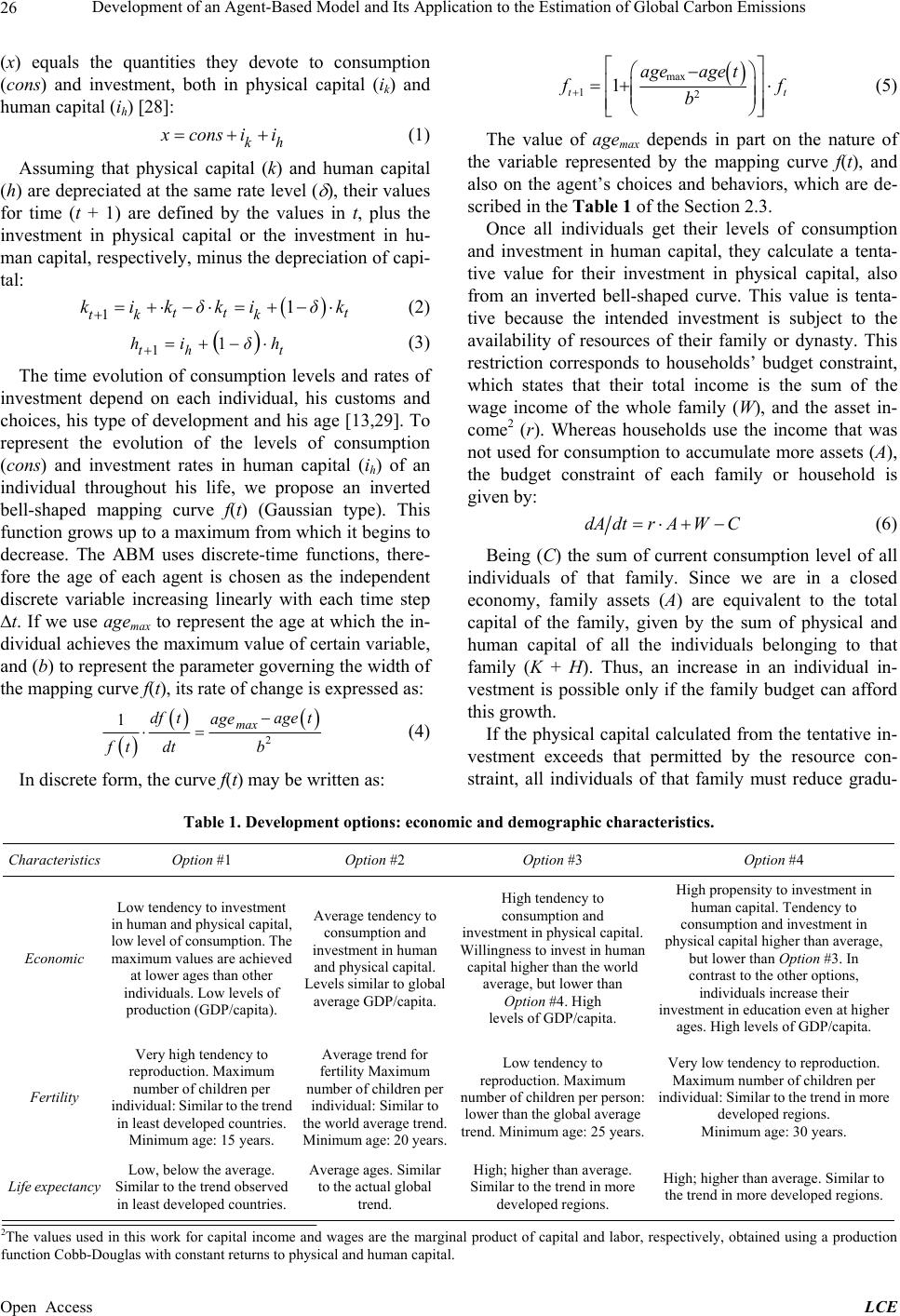 Development of an Agent-Based Model and Its Application to the Estimation of Global Carbon Emissions Open Access LCE 26 (x) equals the quantities they devote to consumption (cons) and investment, both in physical capital (ik) and human capital (ih) [28]: max 12 1 tt ageage t f b (5) kh cons ii (1) The value of agemax depends in part on the nature of the variable represented by the mapping curve f(t), and also on the agent’s choices and behaviors, which are de- scribed in the Table 1 of the Section 2.3. Assuming that physical capital (k) and human capital (h) are depreciated at the same rate level ( ), their values for time (t + 1) are defined by the values in t, plus the investment in physical capital or the investment in hu- man capital, respectively, minus the depreciation of capi- tal: Once all individuals get their levels of consumption and investment in human capital, they calculate a tenta- tive value for their investment in physical capital, also from an inverted bell-shaped curve. This value is tenta- tive because the intended investment is subject to the availability of resources of their family or dynasty. This restriction corresponds to households’ budget constraint, which states that their total income is the sum of the wage income of the whole family (W), and the asset in- come2 (r). Whereas households use the income that was not used for consumption to accumulate more assets (A), the budget constraint of each family or household is given by: 11 tt tkk kikδki δk t (2) t h thδih 1 1 (3) The time evolution of consumption levels and rates of investment depend on each individual, his customs and choices, his type of development and his age [13,29]. To represent the evolution of the levels of consumption (cons) and investment rates in human capital (ih) of an individual throughout his life, we propose an inverted bell-shaped mapping curve f(t) (Gaussian type). This function grows up to a maximum from which it begins to decrease. The ABM uses discrete-time functions, there- fore the age of each agent is chosen as the independent discrete variable increasing linearly with each time step t. If we use agemax to represent the age at which the in- dividual achieves the maximum value of certain variable, and (b) to represent the parameter governing the width of the mapping curve f(t), its rate of change is expressed as: dA dtrAWC (6) Being (C) the sum of current consumption level of all individuals of that family. Since we are in a closed economy, family assets (A) are equivalent to the total capital of the family, given by the sum of physical and human capital of all the individuals belonging to that family (K + H). Thus, an increase in an individual in- vestment is possible only if the family budget can afford this growth. 2 1max dftaget age ft dtb (4) If the physical capital calculated from the tentative in- vestment exceeds that permitted by the resource con- straint, all individuals of that family must reduce gradu- In discrete form, the curve f(t) may be written as: Table 1. Development options: economic and demographic characteristics. Characteristics Option #1 Option #2 Option #3 Option #4 Economic Low tendency to investment in human and physi cal capital, low lev el o f co ns u m p ti on . T h e maximum values are achieved at lower ages than other individuals. Low levels of production (GDP/capita). Average tendency to consumption and investment in human and physical capital. Levels similar to global average GDP/capita. High tendency to consumption and investment in physical capital. Willingness to invest in human capital higher than the world average, but lower than Option #4. High levels of GDP/capita. High propensity to investment in human capital. Tendency to consumption and investment in physical capital higher than average, but lower than Option #3. In contrast to the other options, individuals increase their investment in education even at higher ages. High levels of GDP/capita. Fertility Very high tendency to reproduction. Maximum number of children per indi vidu al: Simi lar t o th e tr end in least developed countries. Minimum age: 15 years. Average trend for fertility Maximum number of children per individual: Similar to the world average trend. Minimum a ge : 2 0 y ea r s. Low tendency to reproduction. Maximum number of children per person: lower than the global average trend. Minimum age: 25 years. Very low tendency to reproduction. Maximum number of children per indi vi du a l: S im i l ar t o t he t re n d in more developed regions. Minimum age: 30 years. Life expectancy Low, below the average. Similar to the trend observed in least developed countries. Average ages. Similar to the actual global trend. High; higher than average. Similar to the trend in more developed regions. High; higher than average. Similar to the trend in more developed regions. 2The values used in this work for capital income and wages are the marginal product of capital and labor, respectively, obtained using a production function Cobb-Douglas with constant returns to physical and human capital. 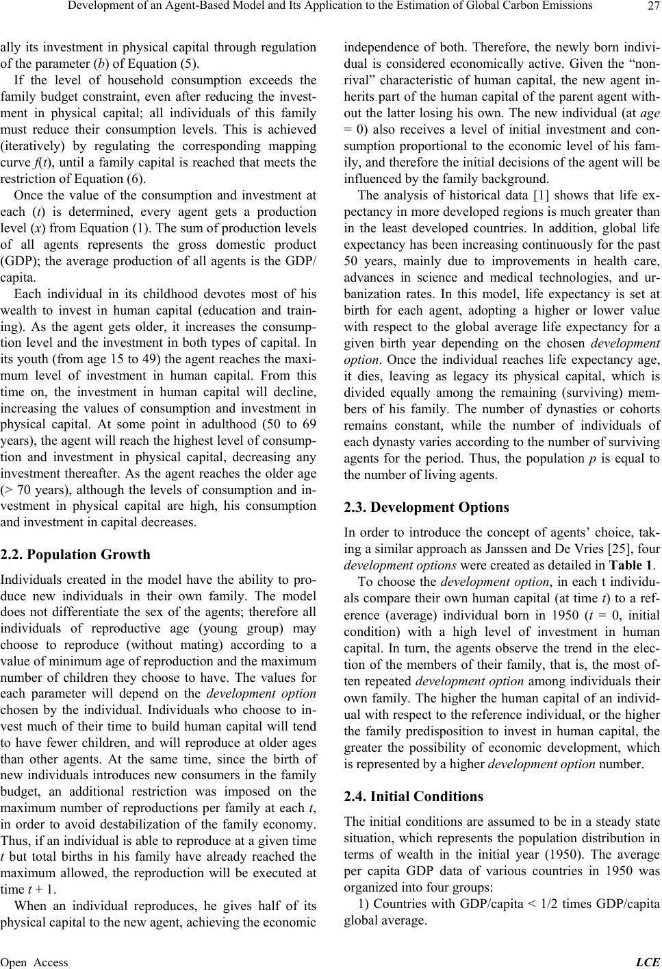 Development of an Agent-Based Model and Its Application to the Estimation of Global Carbon Emissions 27 ally its investment in physical capital through regulation of the parameter (b) of Equation (5). If the level of household consumption exceeds the family budget constraint, even after reducing the invest- ment in physical capital; all individuals of this family must reduce their consumption levels. This is achieved (iteratively) by regulating the corresponding mapping curve f(t), until a family capital is reached that meets the restriction of Equation (6). Once the value of the consumption and investment at each (t) is determined, every agent gets a production level (x) from Equation (1). The sum of production levels of all agents represents the gross domestic product (GDP); the average production of all agents is the GDP/ capita. Each individual in its childhood devotes most of his wealth to invest in human capital (education and train- ing). As the agent gets older, it increases the consump- tion level and the investment in both types of capital. In its youth (from age 15 to 49) the agent reaches the maxi- mum level of investment in human capital. From this time on, the investment in human capital will decline, increasing the values of consumption and investment in physical capital. At some point in adulthood (50 to 69 years), the agent will reach the h ighest level of consump- tion and investment in physical capital, decreasing any investment thereafter. As the agent reaches the older age (> 70 years), although the levels of consumption and in- vestment in physical capital are high, his consumption and investment in capital decreases. 2.2. Population Growth Individuals created in the model have the ability to pro- duce new individuals in their own family. The model does not differentiate the sex of the agents; therefore all individuals of reproductive age (young group) may choose to reproduce (without mating) according to a value of minimum age of reproduction and the maximum number of children they choose to have. The values for each parameter will depend on the development option chosen by the individual. Individuals who choose to in- vest much of their time to build human capital will tend to have fewer children, and will reproduce at older ages than other agents. At the same time, since the birth of new individuals introduces new consumers in the family budget, an additional restriction was imposed on the maximum number of reproductions per family at each t, in order to avoid destabilization of the family economy. Thus, if an individual is able to reproduce at a given time t but total births in his family have already reached the maximum allowed, the reproduction will be executed at time t + 1. When an individual reproduces, he gives half of its physical capital to the new agent, achieving the economic independence of both. Therefore, the newly born indivi- dual is considered economically active. Given the “non- rival” characteristic of human capital, the new agent in- herits part of the human capital of the parent agent with- out the latter losing his own. The new individual (at age = 0) also receives a level of initial investment and con- sumption proportional to the economic level of his fam- ily, and therefore the initial decision s of the agent will b e influenced by the family backgroun d. The analysis of historical data [1] shows that life ex- pectancy in more developed regions is much greater than in the least developed countries. In addition, global life expectancy has been increasing continuously for the past 50 years, mainly due to improvements in health care, advances in science and medical technologies, and ur- banization rates. In this model, life expectancy is set at birth for each agent, adopting a higher or lower value with respect to the global average life expectancy for a given birth year depending on the chosen development option. Once the individual reaches life expectancy age, it dies, leaving as legacy its physical capital, which is divided equally among the remaining (surviving) mem- bers of his family. The number of dynasties or cohorts remains constant, while the number of individuals of each dynasty varies according to the number of surviving agents for the period. Thus, the population p is equal to the number of living agents. 2.3. Development Options In order to introduce the concept of agents’ choice, tak- ing a similar approach as Janssen and De Vries [25], four development options were created as detailed in Table 1. To choose the development option, in each t individu- als compare their own human capital (at time t) to a ref- erence (average) individual born in 1950 (t = 0, initial condition) with a high level of investment in human capital. In turn, the agents observe the trend in the elec- tion of the members of their family, that is, the most of- ten repeated development option among individuals their own family. The higher the human capital of an individ- ual with respect to the reference individual, or the higher the family predisposition to invest in human capital, the greater the possibility of economic development, which is represented by a higher development option number. 2.4. Initial Conditions The initial conditions are assumed to be in a steady state situation, which represents the population distribution in terms of wealth in the initial year (1950). The average per capita GDP data of various countries in 1950 was organized into four groups: 1) Countries with GDP/capita < 1/2 times GDP/capita global average. Open Access LCE 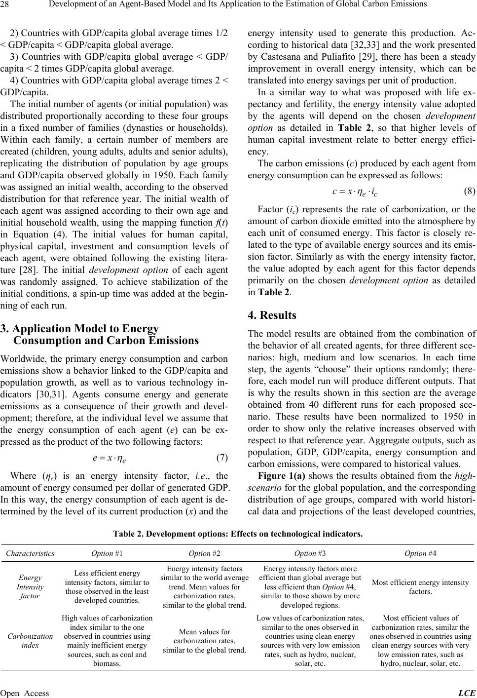 Development of an Agent-Based Model and Its Application to the Estimation of Global Carbon Emissions 28 2) Countries with GDP/capita global average times 1/2 < GDP/capita < GDP/capita global average. 3) Countries with GDP/capita global average < GDP/ capita < 2 times GDP/capita global averag e. 4) Countries with GDP/capita global average times 2 < GDP/capita. The initial number of agents (or initial popu lation) was distributed proportionally according to these four groups in a fixed number of families (dynasties or households). Within each family, a certain number of members are created (children, young adults, adults and senior adults), replicating the distribution of population by age groups and GDP/capita observed globally in 1950. Each family was assigned an initial wealth, according to the observed distribution for that reference year. The initial wealth of each agent was assigned according to their own age and initial household wealth, using the mapping function f(t) in Equation (4). The initial values for human capital, physical capital, investment and consumption levels of each agent, were obtained following the existing litera- ture [28]. The initial development option of each agent was randomly assigned. To achieve stabilization of the initial condition s, a spin-up time was added at the begin- ning of each run. 3. Application Model to Energy Consumption and Carbon Emissions Worldwide, the primary energy consumption and carbon emissions show a behavior linked to the GDP/capita and population growth, as well as to various technology in- dicators [30,31]. Agents consume energy and generate emissions as a consequence of their growth and devel- opment; therefore, at the individual level we assume that the energy consumption of each agent (e) can be ex- pressed as the product of the two following factors: e ex (7) Where (ηe) is an energy intensity factor, i.e., the amount of energy consumed per dollar of generated GDP. In this way, the energy consumption of each agent is de- termined by the level of its current production (x) and the energy intensity used to generate this production. Ac- cording to historical data [32,33] and the work presented by Castesana and Puliafito [29], there has been a steady improvement in overall energy intensity, which can be translated into energy savings per unit of production. In a similar way to what was proposed with life ex- pectancy and fertility, the energy intensity value adopted by the agents will depend on the chosen development option as detailed in Table 2, so that higher levels of human capital investment relate to better energy effici- ency. The carbon emissions (c) produced by each agent from energy consumption can be expressed as follows: ec cx i (8) Factor (ic) represents the rate of carbonization, or the amount of carbon dioxide emitted into the atmosphere by each unit of consumed energy. This factor is closely re- lated to the type of available en ergy sour ces and its emis- sion factor. Similarly as with the energy intensity factor, the value adopted by each agent for this factor depends primarily on the chosen development option as detailed in Table 2. 4. Results The model results are obtained from the combination of the behavior of all created agents, for three different sce- narios: high, medium and low scenarios. In each time step, the agents “choose” their options randomly; there- fore, each model run will produce different outputs. That is why the results shown in this section are the average obtained from 40 different runs for each proposed sce- nario. These results have been normalized to 1950 in order to show only the relative increases observed with respect to that reference year. Aggregate outputs, such as population, GDP, GDP/capita, energy consumption and carbon emissions, were compared to historical values. Figure 1(a) shows the results obtained from the high- scenario for the global population, and the corresponding distribution of age groups, compared with world histori- cal data and projections of the least developed countries, Table 2. Development options: Effects on technological indicators. Characteristics Option #1 Option #2 Option #3 Option #4 Energy Intensity factor Less efficient energy intensity factors, similar to those observed in the least developed countries. Energy intensity factors similar to the world average trend. Mean values for carbonization rates, similar to the global trend. Energy intensity factors more efficient than global average but less efficient than Option #4, similar to those shown by more developed regions. Most efficient energy intensity factors. Carbonization index High v a l u e s o f c a rbon i z a t i o n index similar to the one observed in countries using mainly inefficient energy sources, such as coal and biomass. Mean values for carbonization rates, similar to the global trend. Low value s of car boniza tion rate s, similar to the ones observed in countries using clean energy sources with very low emission rates, such as hydro, nuclear, solar, etc. Most efficient values of carbonization rates, similar the ones obs erv ed i n c ount rie s us ing clean energy sources with very low emission rates, such as hydro, nuclear, solar, etc. Open Access LCE 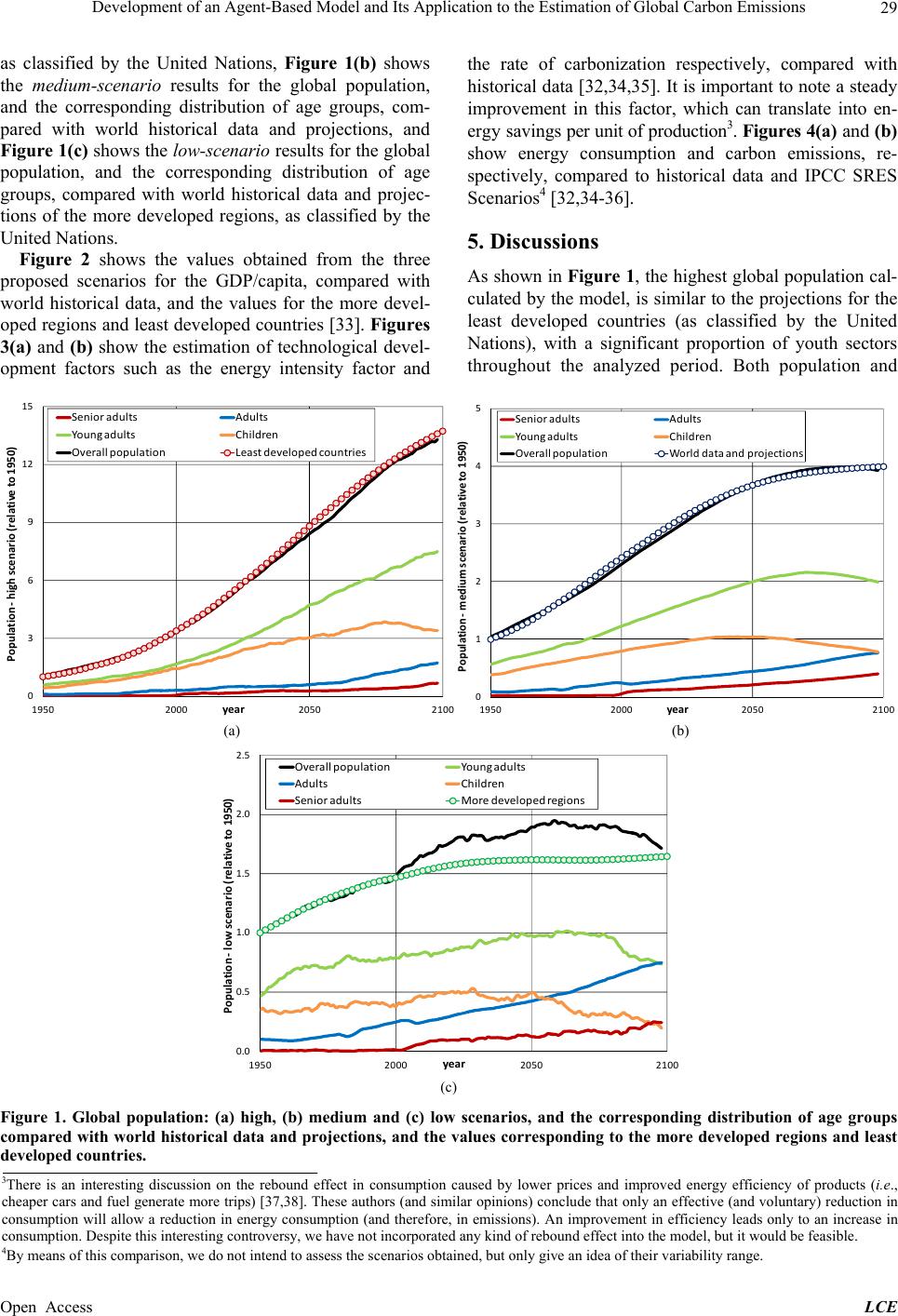 Development of an Agent-Based Model and Its Application to the Estimation of Global Carbon Emissions 29 as classified by the United Nations, Figure 1(b) shows the medium-scenario results for the global population, and the corresponding distribution of age groups, com- pared with world historical data and projections, and Figure 1(c) shows th e low-scenario results for the global population, and the corresponding distribution of age groups, compared with world historical data and projec- tions of the more developed regions, as classified by the United Nations. Figure 2 shows the values obtained from the three proposed scenarios for the GDP/capita, compared with world historical data, and the values for the more devel- oped regions and least developed countries [33]. Figures 3(a) and (b) show the estimation of technological devel- opment factors such as the energy intensity factor and the rate of carbonization respectively, compared with historical data [32,34,35]. It is important to note a steady improvement in this factor, which can translate into en- erg y sav ings per unit of production3. Figures 4(a) and (b) show energy consumption and carbon emissions, re- spectively, compared to historical data and IPCC SRES Scenarios4 [32,34-36]. 5. Discussions As shown in Figure 1, the highest global population cal- culated by the model, is similar to the projections for the least developed countries (as classified by the United Nations), with a significant proportion of youth sectors throughout the analyzed period. Both population and 0 3 6 9 12 15 1950 2000 2050 2100 Population‐ highscenario(relativeto1950) ear Senioradults Adults Youngadults Children Overall populationLeastdevelopedcountries (a) 0 1 2 3 4 5 1950 2000 2050 2100 Population‐ mediumscenario(relativeto 1950) yea r Senio radults Adults Youngadults Children Overall population Worlddataandprojections (b) (a) (b) 0.0 0.5 1.0 1.5 2.0 2.5 1950 2000 2050 2100 Population‐ lowscenario(relativeto 1950) yea r Overallpopulation Young adults Adults Chil d ren SenioradultsMoredevelopedregio n s (c) (c) Figure 1. Global population: (a) high, (b) medium and (c) low scenarios, and the corresponding distribution of age groups compared with world historical data and projections, and the values corresponding to the more developed regions and least developed countrie s. 3There is an interesting discussion on the rebound effect in consumption caused by lower prices and improved energy efficiency of products (i.e., cheaper cars and fuel generate more trips) [37,38]. These authors (and similar opinions) conclude that only an effective (and voluntary) reduction in consumption will allow a reduction in energy consumption (and therefore, in emissions). An improvement in efficiency leads only to an increase in consumption. Despite this interesting controversy, we have not incorporated any kind of rebound effect into the model, but it would be feasible. 4By means of this comparison, we do not intend to assess the scenarios obtained, but only give an idea of their variability range. Open Access LCE 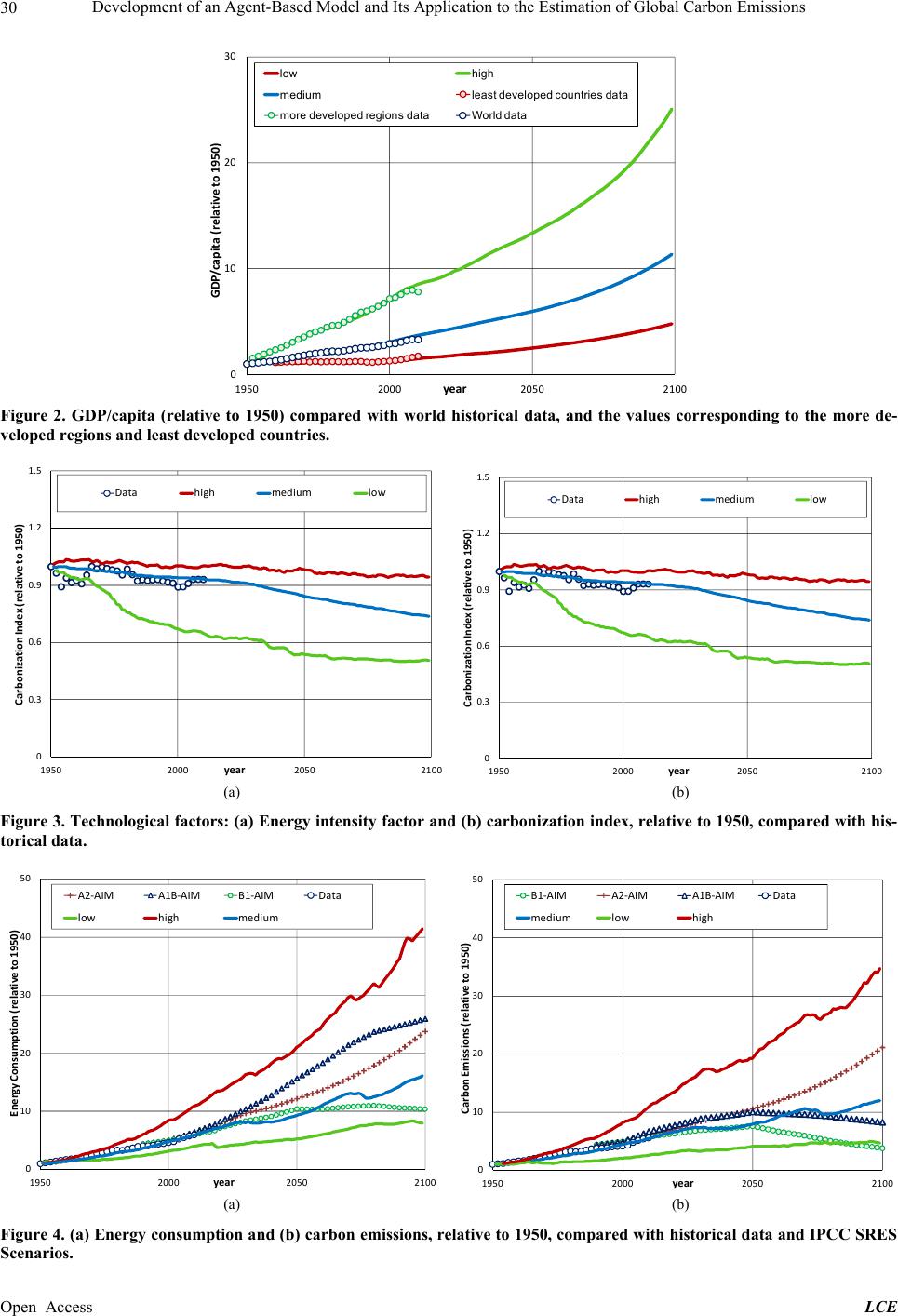 Development of an Agent-Based Model and Its Application to the Estimation of Global Carbon Emissions 30 0 10 20 30 1950 2000 2050 2100 GDP/capita(relativeto1950) ear low high medium least developed countries data more developed regions dataWorld data Figure 2. GDP/capita (relative to 1950) compared with world historical data, and the values corresponding to the more de- veloped regions and least develope d c ountries. 0 0.3 0.6 0.9 1.2 1.5 1950200020502100 0 0.3 0.6 0.9 1.2 1.5 1950 2000 2050 2100 CarbonizationIndex(relativeto1950) ear Data high mediumlow (b) Data Carbon iz ationIndex (relativeto1950) year high medium low (b ) (a) (b) Figure 3. Technological factors: (a) Energy intensity factor and (b) carbonization index, relative to 1950, compared with his- torical data. 0 10 20 30 40 50 1950 2000 2050 2100 EnergyConsumption(relativeto1950) year A2‐AIM A1B‐AIM B1‐AIM Data low high medium (a) 0 10 20 30 40 50 1950 2000 2050 2100 CarbonEmissions(relativeto1950) year B1‐AIM A2‐AIM A1B‐AIMData medium low high (b) (a) (b) Figure 4. (a) Energy consumption and (b) carbon emissions, relative to 1950, compared with historical data and IPCC SRES Scenarios. Open Access LCE 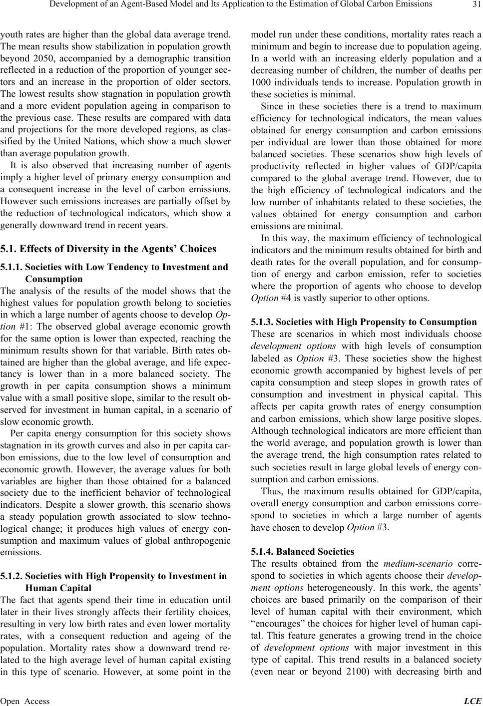 Development of an Agent-Based Model and Its Application to the Estimation of Global Carbon Emissions Open Access LCE 31 youth ra tes are higher than the global data ave rage trend. The mean results show stabilization in pop ulation growth beyond 2050, accompanied by a demographic transition reflected in a reduction of the proportion of younger sec- tors and an increase in the proportion of older sectors. The lowest results show stagnation in population growth and a more evident population ageing in comparison to the previous case. These results are compared with data and projections for the more developed regions, as clas- sified by the United Natio ns, which show a much slower than average po pulation growth. It is also observed that increasing number of agents imply a higher level of primary energy consumption and a consequent increase in the level of carbon emissions. However such emissions increases are partially offset by the reduction of technological indicators, which show a generally downward trend in recent years. 5.1. Effects of Diversity in the Agents’ Choices 5.1.1. Societies with Low Tendency to Investment and Consumption The analysis of the results of the model shows that the highest values for population growth belong to societies in which a large number of agents choose to develop Op- tion #1: The observed global average economic growth for the same option is lower than expected, reaching the minimum results shown for that variable. Birth rates ob- tained ar e higher than the g lobal average , and life expec- tancy is lower than in a more balanced society. The growth in per capita consumption shows a minimum value with a small positiv e slope, similar to th e result ob- served for investment in human capital, in a scenario of slow economic growth. Per capita energy consumption for this society shows stagnation in its g rowth curves and also in per capita car- bon emissions, due to the low level of consumption and economic growth. However, the average values for both variables are higher than those obtained for a balanced society due to the inefficient behavior of technological indicators. Despite a slower growth, this scenario shows a steady population growth associated to slow techno- logical change; it produces high values of energy con- sumption and maximum values of global anthropogenic emissions. 5.1.2. Societies with High Propensity to Investment in Human Capital The fact that agents spend their time in education until later in their lives strongly affects their fertility choices, resulting in very low birth rates and even lower mortality rates, with a consequent reduction and ageing of the population. Mortality rates show a downward trend re- lated to the high average level of human capital existing in this type of scenario. However, at some point in the model run under these conditions, mortality rates reach a minimum and begin to increase due to population ageing. In a world with an increasing elderly population and a decreasing number of children, the number of deaths per 1000 individuals tends to increase. Population growth in these societies is minimal. Since in these societies there is a trend to maximum efficiency for technological indicators, the mean values obtained for energy consumption and carbon emissions per individual are lower than those obtained for more balanced societies. These scenarios show high levels of productivity reflected in higher values of GDP/capita compared to the global average trend. However, due to the high efficiency of technological indicators and the low number of inhabitants related to these societies, the values obtained for energy consumption and carbon emissions are minimal. In this way, the maximum efficiency of technological indicators and the minimum results obtained for birth and death rates for the overall population, and for consump- tion of energy and carbon emission, refer to societies where the proportion of agents who choose to develop Option #4 is vastly superior to other options. 5.1.3. Societies with High Propensity to Consumption These are scenarios in which most individuals choose development options with high levels of consumption labeled as Option #3. These societies show the highest economic growth accompanied by highest levels of per capita consumption and steep slopes in growth rates of consumption and investment in physical capital. This affects per capita growth rates of energy consumption and carbon emissions, which show large positive slopes. Although techno logical indicators are more efficient than the world average, and population growth is lower than the average trend, the high consumption rates related to such societies result in large global levels of energ y con- sumption and carbon emissions. Thus, the maximum results obtained for GDP/capita, overall energy consumption and carbon emissions corre- spond to societies in which a large number of agents have chosen to develop Option #3. 5.1.4. Balanced Societies The results obtained from the medium-scenario corre- spond to societies in which agents choose their develop- ment options heterogeneously. In this work, the agents’ choices are based primarily on the comparison of their level of human capital with their environment, which “encourages” the choices for higher level of human capi- tal. This feature generates a growing trend in the choice of development options with major investment in this type of capital. This trend results in a balanced society (even near or beyond 2100) with decreasing birth and 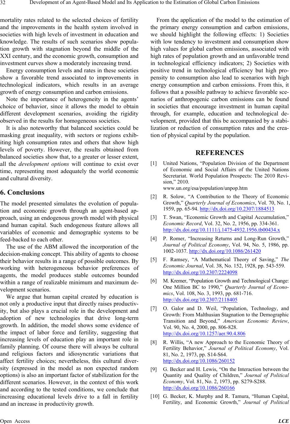 Development of an Agent-Based Model and Its Application to the Estimation of Global Carbon Emissions 32 mortality rates related to the selected choices of fertility and the improvements in the health system involved in societies with high levels of investment in education and knowledge. The results of such scenarios show popula- tion growth with stagnation beyond the middle of the XXI century, and the economic growth, consumption and investment curves show a moderately increasing trend. Energy consumption levels and rates in these societies show a favorable trend associated to improvements in technological indicators, which results in an average growth of energy consumption and carbon emissions. Note the importance of heterogeneity in the agents’ choice of behavior, since it allows the model to obtain different development scenarios, avoiding the rigidity observed in the results for homogeneous societies. It is also noteworthy that balanced societies could be masking great inequality, with sectors or regions exhib- iting high consumption rates and others that show high levels of poverty. However, the results obtained from balanced societies show th at, to a greater or lesser extent, all the development options will continue to exist over time, representing most adequately the world economic and cultural diversity. 6. Conclusions The model presented simulates the evolution of popula- tion and economic growth through an agent-based ap- proach, using an endogenous growth model with physical and human capital. Such endogenous feature allows all variables of economic and demographic systems to be feed-backed to each other. The use of the ABM allowed the incorporation of the decision-making concept. This ab ility of agen ts to cho ose their behavior results in a range of possible outcomes. By working with heterogeneous behavior preferences of agents, the model produces stable outcomes bounded within a range of realizable minimum and maximum de- velopment scenarios. We argue that human capital created by education is not only a productive input that directly raises productiv- ity, but also plays a crucial role in the development and adoption of new technologies that drive long-term growth. In addition, the model shows some evidence of the impact of labor force and fertility, suggesting that increasing levels of education play an important role in family planning. Of course there will always be cultural and religious factors and idiosyncratic variations that affect fertility choices; nevertheless, this cultural diver- sity (expressed in the model as non expected random options) is also an important factor of stabilization for the different scenarios. However, in the context of this work and according to the tested conditions, we conclude that increasing educational levels drive to a fall in fertility and an increase in productivity growth. From the application of the model to the estimation of the primary energy consumption and carbon emissions, we should highlight the following effects: 1) Societies with low tendency to investment and consumption show high values for global carbon emissions, associated with high rates of popu lation growth and an unfavor able trend in technological efficiency indicators; 2) Societies with positive trend in technological efficiency but high pro- pensity to consumption also lead to scenarios with high energy consumption and carbon emissions. From this, it follows that a possible pathway to achieve favorable sce- narios of anthropogenic carbon emissions can be found in societies that encourage investment in human capital through, for example, education and technological de- velopment, provided that this be accompanied by a stabi- lization or reduction of consumption rates and the crea- tion of physical capital by th e population. REFERENCES [1] United Nations, “Population Division of the Department of Economic and Social Affairs of the United Nations Secretariat. World Population Prospects: The 2010 Revi- sion,” 2010. www.un.org/esa/population/unpop.htm [2] R. Solow, “A Contribution to the Theory of Economic Growth,” Quarterly Journal of Economics, Vol. 70, No. 1, 1959, pp. 65-94. http://dx.doi.org/10.2307/1884513 [3] T. Swan, “Economic Growth and Capital Accumulation,” Economic Record, Vol. 32, No. 2, 1956, pp. 334-361. http://dx.doi.org/10.1111/j.1475-4932.1956.tb00434.x [4] P. Romer, “Increasing Returns and Long-Run Growth,” Journal of Political Economy, Vol. 94, No. 5, 1986, pp. 1002-1037. http://dx.doi.org/10.1086/261420 [5] F. Ramsey, “A Mathematical Theory of Saving,” The Economic Journal, Vol. 38, No. 152, 1928, pp. 543-559. http://dx.doi.org/10.2307/2224098 [6] M. Kremer, “Populati on Growth and Techno logical Change : One Million BC to 1990,” Quarterly Journal of Econo- mics, Vol. 108, No. 3, 1993, pp. 681-716. http://dx.doi.org/10.2307/2118405 [7] O. Galor and D. Weil, “Population, Technology, and Growth: From Malthusian Stagnation to the Demographic Transition and Beyond,” American Economic Review, Vol. 90, No. 4, 2000, pp. 806-828. http://dx.doi.org/10.1257/aer.90.4.806 [8] R. Willis, “A new Approach to the Economic Theory of Fertility Behavior,” Journal of Political Economy, Vol. 81, No. 2, 1973, pp. S14-S64. http://dx.doi.org/10.1086/260152 [9] G. Becker and H. Lewis, “On the Interaction between the Quantity and Quality of Children,” Journal of Political Economy, Vol. 81, No. 2, 1973, pp. S279-S288. http://dx.doi.org/10.1086/260166 [10] G. Becker, K. Murphy and R. Tamura, “Human Capital, Fertility, and Economic Growth,” Journal of Political Open Access LCE  Development of an Agent-Based Model and Its Application to the Estimation of Global Carbon Emissions 33 Economy, Vol. 98, No. 5, 1990, pp. S12-S37. http://dx.doi.org/10.1086/261723 [11] O. Galor and D. Weil, “The Gender Gap, Fertility, and Growth,” American Economic Review, Vol. 86, No. 3, 1996, pp. 374-387. [12] C. Jones, “R&D-Based Models of Economic Growth,” Journal of Political Economy, Vol. 103, No. 4, 1995, pp. 759-784. http://dx.doi.org/10.1086/262002 [13] R. Lee and A. Mason, “Some Macroeconomic Aspects of Global Population Aging,” Demography, Vol. 47 Suppl, 2010, pp. S151-S172. http://dx.doi.org/10.1353/dem.2010.0002 [14] C. Day and S. Dowrick, “Ageing Economics: Human Capital, Productivity and Fertility,” Agenda, Vol. 11, No. 1, 2004, pp. 3-20. [15] N. Jennings, K. Sycara and M. Wooldridge, “A Roadmap of Agent Research and Development,” Autonomous Agents and Multi-Agent Systems, Vol. 1, No. 1, 1998, pp. 7-38. http://dx.doi.org/10.1023/A:1010090405266 [16] M. Wooldridge and N. Jennings, “Software Engineering with Agents: Pitfalls and Pratfalls,” Internet Computing, Vol. 3, No. 3, 1999, pp. 20-27. http://dx.doi.org/10.1109/4236.769419 [17] E. Bonabeau, “Agent-Based Modeling: Methods and Techniques for Simulating Human Systems,” Proceed- ings of the National Academy of Sciences of the United States of America, Vol. 99, 2002, pp. 7280-7287. http://dx.doi.org/10.1073/pnas.082080899 [18] B. Edmonds, “The Use of Models—Making MABs More Informative,” Multi-Agent-Based Simulation, Vol. 1979, No. 1979, 2001, pp. 15-32. [19] H. Kelley and T. Evans, “The Relative Influences of Land-Owner and Landscape Heterogeneity in an Agent- Based Model of Land-Use,” Ecological Economics, Vol. 70, No. 6, 2011, pp. 1075-1087. http://dx.doi.org/10.1016/j.ecolecon.2010.12.009 [20] F. Bert, G. Podestá, S. Rovere, Á. Menéndez, M. North, E. Tatara, C. Laciana, E. Weber and F. Ruiz Toranzo, “An Agent Based Model to Simulate Structural and Land Use Changes in Agricultural Systems of the Argentine Pam- pas,” Ecological Modelling, Vol. 222, No. 19, 2011, pp. 3486-3499. http://dx.doi.org/10.1016/j.ecolmodel.2011.08.007 [21] R. Damaceanu, “An Agent-Based Computational Study of Wealth Distribution in Function of Resource Growth Interval Using Netlogo,” Applied Mathematics and Com- putation, Vol. 201, No. 1-2, 2008, pp. 371-377. http://dx.doi.org/10.1016/j.amc.2007.12.042 [22] M. Vaz Martins, T. Araujo, M. Santos and M. Aubyn, “Network Effects in a Human Capital Based Economic Growth Model,” Quantitative Finance, Vol. 388, 2009, pp. 2207-2214. [23] S. Natarajan, J. Padget and L. Elliott, “Modelling UK Domestic Energy and Carbon Emissions: An Agent- Based Approach,” Energy and Buildings, Vol. 43, No. 10, 2011, pp. 2602-2612. http://dx.doi.org/10.1016/j.enbuild.2011.05.013 [24] E. Chappin and G. Dijkema, “On the Impact of CO2 Emission-Trading on Power Generation Emissions,” Tech- nological Forecasting and Social Change, Vol. 76, No. 3, 2009, pp. 358-370. http://dx.doi.org/10.1016/j.techfore.2008.08.004 [25] M. Janssen and B. De Vries, “The Battle of Perspectives: a Multi-Agent Model with Adaptive Responses to Cli- mate Change,” Ecological Economics, Vol. 26, 1998, pp. 43-65. http://dx.doi.org/10.1016/S0921-8009(97)00062-1 [26] F. Schweitzer, G. Fagiolo, D. Sornette, F. Vega-Redondo, A. Vespignani and D. R. White, “Economic Networks: The New Challenges,” Science, Vol. 325, No. 5939, 2009, pp. 422-425. [27] J. Farmer and D. Foley, “The Economy Needs Agent- Based Modelling,” Nature, Vol. 460, No. 7256, 2009, pp. 685-686. http://dx.doi.org/10.1038/460685a [28] R. Barro and X. Sala-i-Martin, “Two-Sector Models of Endogenous Growth (with Special Attention to the Role of Human Capital),” In: R. Barro and X. Sala-i-Martin, Eds., Economic Growth, 2nd Edition, The MIT Press, Cambridge, 2004, pp. 239-284. [29] P. Castesana and S. Puliafito, “Bottom-Up Analysis of Energy Consumption and Carbon Emissions, with Par- ticular Emphasis on Human Capital Investment,” Low- Carbon Economy, Vol. 4, No. 4A2, 2013. [30] E. Puliafito, J. Puliafito and M. Conte Grand, “Modeling Population Dynamics and Economic Growth as Compet- ing Species: An Application to CO2 Global Emissions,” Ecological Economics, Vol. 65, No. 3, 2008, pp. 602-615. http://dx.doi.org/10.1016/j.ecolecon.2007.08.010 [31] M. Raupach, J. Canadell and C. Le Quéré, “Anthropo- genic and Biophysical Contributions to Increasing At- mospheric CO2 Growth Rate and Airborne Fraction,” Biogeosciences, Vol. 5, No. 6, 2008, pp. 1601-1613. http://dx.doi.org/10.5194/bg-5-1601-2008 [32] British Petroleum, “British Petroleum Statistical Review of World Energy June 2012,” London, 2012. www.bp.com/statisticalreview [33] World Bank, “World Bank Database,” World Develop- ment Indicators (WDI) and Global Development Finance (GDF), Washington DC, 2011. http://databank.worldbank.org/ [34] T. Boden, G. Marland and R. Andres, “Global, Regional, and National Fossil-Fuel CO2 Emissions. Carbon Dioxide Information Analysis Center, Oak Ridge National Labo- ratory,” US Department of Energy, Oak Ridge, 2011. [35] A. Grubler, “Energy Transitions,” In: C. Cleveland, Ed., Encyclopedia of Earth, Environmental Information Coali- tion, National Council for Science and the Environment, Washington DC, 2008. www.eoearth.org/view/article/152561/ [36] N. Nakicenovic, J. Alcamo, G. Davis, B. De Vries, J. Fenhann, S. Gaffin, K. Gregory, A. Grubler, T. Jung, T. Kram, E. La Rovere, L. Michaelis, S. Mori, T. Morita, W. Pepper, H. Pitcher, L. Price, K. Raihi, A. Roehrl, H. Rogner, A. Sankovski, M. Schlesinger, P. Shukla, S. Smith, R. Swart, S. Van Rooijen, N. Victor and Z. Dadi, “IPCC Special Report on Emissions Scenarios (SRES),” Cambridge University Press, Cambridge, 2000, p. 595. Open Access LCE  Development of an Agent-Based Model and Its Application to the Estimation of Global Carbon Emissions Open Access LCE 34 [37] R. Madlener and B. Alcott, “Energy Rebound and Eco- nomic Growth: A Review of the Main Issues and Re- search Needs,” Energy, Vol. 34, No. 3, 2009, pp. 370-376. http://dx.doi.org/10.1016/j.energy.2008.10.011 [38] S. Sorrell, “The Rebound Effect: An Assessment of the Evidence for Economy-Wide Energy Savings from Im- proved Energy Efficiency,” Sussex Energy Group for the Technology and Policy Assessment Function of the UK Energy Research Centre, London, 2007. http://www.ukerc.ac.uk/Downloads/PDF/07/0710Reboun dEffect/0710ReboundEffectReport.pdf
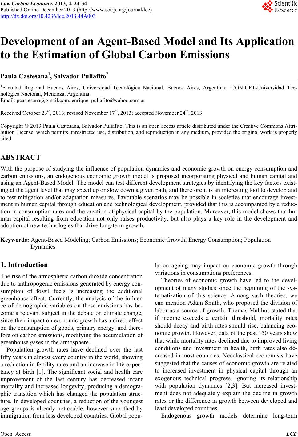
|