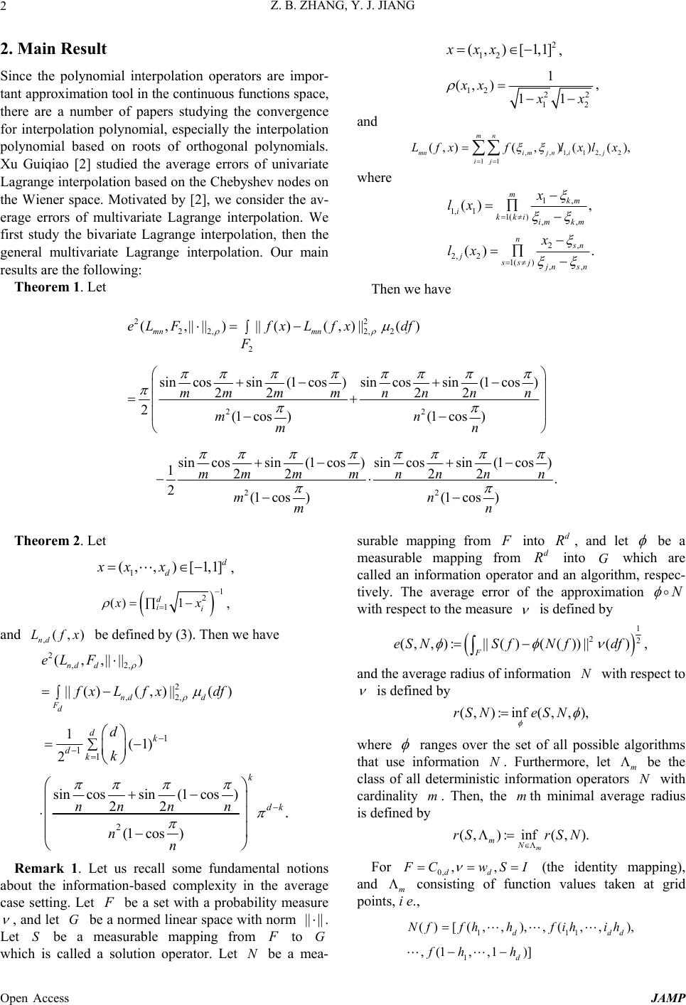
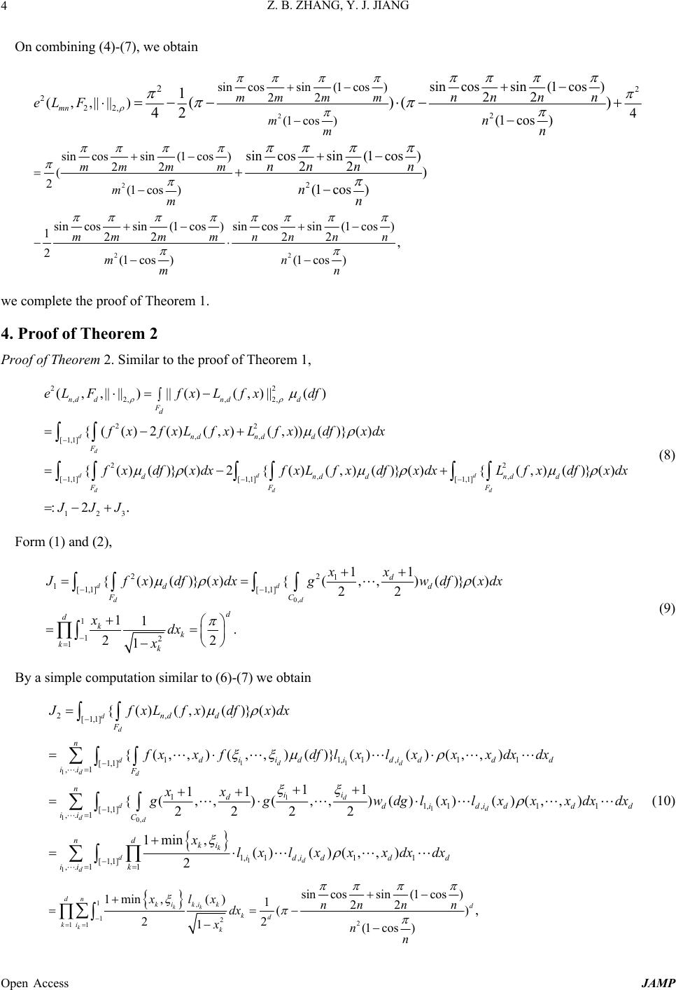
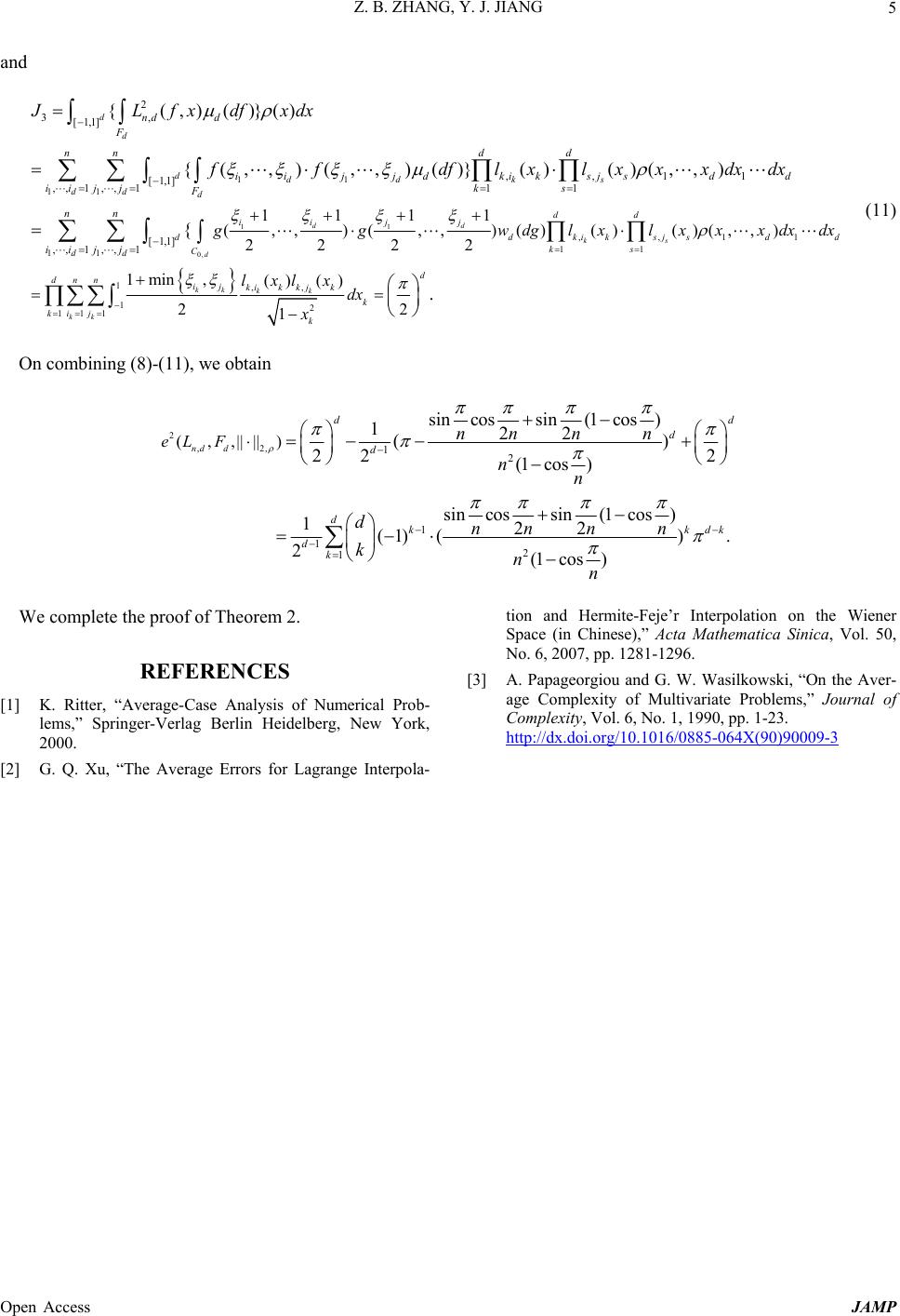
J
ournal o
f
A
pp
Published Onli
n
http://dx.doi.or
g
Open Access
ABSTRA
C
In this
p
aper,
first kind. Th
e
Keywords:
M
1. Introdu
c
Let F
b
e a
r
a probability
X
b
e another
embedded in
Any :TF

measurable
m
The average
e
(,eT
F
For 1d ,
0,d
C
The space
The classic
is Gaussian
w
(
,
d
w
Rs
For more
d
we refer to [1
]
In this pap
e
*
Supported by N
a
no. 10871132 a
n
higher school sci
e
#
Corresponding
a
p
lied Mathemat
i
n
e November 2
0
g
/10.4236/jamp
.
On
Department
o
C
T
we discuss th
e
e
average erro
r
M
ultivariate L
a
c
tion
r
eal separable
measure

o
normed spac
e
X
. By || ||
X

X

such t
h
m
apping is call
e
e
rror of
T
is
d
,||||):||
XF
Ff




le
t
{[0,1]|
whenever
d
i
fC
f
x


0,d
C equippe
d
[
|| || s
u
t
f


al Wiener sh
e
w
ith mean zero
0,
1
,
)()
min{
,
d
C
d
i
i
tfs
f
s





d
etailed disc
u
]
.
e
r, we le
t
a
tional Natural S
c
n
d 11271263) a
n
e
nce and technol
o
a
utho
r
.
i
cs and Ph
y
sics
,
0
13 (http://ww
w
.2013.16001
the Av
e
La
g
o
f Mathematics
e
average erro
r
r
s of the inter
p
a
grange Int erp
o
Banach spac
e
o
n the Borel
e
such that
F
we denote t
h
h
at ||
f
f


e
d an approxi
m
d
efined as
2
()||
(
X
f
Tf


1
(, ,)
0for some 1
d
f
xx


d
with the sup
0,1]
u
p| ()|
d
ft .
e
et measure
w
and covarian
c
()( )
,
}, ,
d
i
f
tw df
tst
u
ssion and pr
o
c
ience Foundatio
n
n
d by a grant fr
o
o
gy research (Z20
1
,
2013, 1, 1-5
w
.scirp.org/jour
n
e
rage
E
g
range
Zengbo Z
h
and Physics, N
o
#
j
Rece
r
s of multivar
i
olation seque
n
o
lation; Avera
g
e
equippe
d
wi
t
sets of
F
.
L
is continuous
l
h
e norm in
X
()||
X
Tf

is
m
ation operat
o
1/2
(
).df 


0,
}.id
nor
m
d
w
on
0,
(
d
C B
c
e kernel
[0,1] .
d
(
o
perties of
d
w
n
of China (Proj
e
o
m Hebei provin
c
1
0160).
n
al
/
jamp )
E
rrors
o
Interp
o
h
ang, Yanjie
o
rth China Elec
t
j
o
ive
d
July 2013
i
ate Lagrange
i
n
ce are deter
m
g
e Error; Che
b
t
h
L
e
t
ly
X
.
a
o
r.
)
d
1)
d
,
For
the me
a
Let
norm f
o
Let
is the
z
Cheby
s
well-k
n
b
ased
o
where
e
c
t
c
e
o
f Mult
i
o
lation
*
Jiang
#
t
ric Power Uni
v
om
i
nterpolation
b
m
ined on the m
u
b
yshev Polyn
o
1
{
(2
d
F
f
f
x


every measu
r
a
sure of A by
1
():
(2
d
A
f
x



1
(, , )
d
x
x 


or
d
f
F is
2,
|| ||:||||
f
f

,
::
kkn


z
eros of ()
n
Tx
s
hev polynom
i
n
own Lagran
g
o
n


1
,,
d
ii


1
,
,, 1
(,)
(
d
nd
n
ii
Lfx
f




,
()
j
ji jk
lx

i
variat
e
*
v
ersity, Baoding
,
b
ased on the
C
u
ltivariate Wi
e
o
mial; Wiener
[1,1]|
(
1,, 21
)
d
d
Cg
x



 
r
able subse
t
A
1
1
{( ,,
1,,2
1
d
d
wgx
x





2
1
1
d
i
i
x




defined as
[1,1]
:|(
)
d
ft







21
cos ,
2
k
n



cos (nx



i
al of the first
g
e interpolati
o

1
,, 1
d
n
ii
is giv
e
11
1, 1
,)(
)
d
iii
lx

 
1( )
,
jj
n
j
k
ki ik
x







e
,
China
C
hebyshev no
d
e
ner space.
Sheet Measur
e
1
0,
(
,,)
)
}.
d
d
xx
C

()
d
A
F B , w
)
1
)}.
d
x
A

1
, the weig
h
1/2
2
)
|() .tdt 




1, , kn
cos )  , the n t
h
kind. For
f

o
n polynomi
a
e
n b
y
,
)
(),
d
di d
lx
,
1,, .jd
JAMP
d
es of the
e
w
e define
(2)
h
ted
2
L -
t
h degree
d
F

, the
a
l of
f
(3)

Z. B. ZHANG, Y. J. JIANG
Open Access JAMP
2
2. Main Result
Since the polynomial interpolation operators are impor-
tan t app rox imation tool in the continuous functions spa ce,
there are a number of papers studying the convergence
for interpolation polynomial, especially the interpolation
polynomial based on roots of orthogonal polynomials.
Xu Guiqiao [2] studied the average errors of univariate
Lagrange interpolation based on the Chebyshev nodes on
the Wiener space. Motivated by [2], we consider the av-
erage errors of multivariate Lagrange interpolation. We
first study the bivariate Lagrange interpolation, then the
general multivariate Lagrange interpolation. Our main
results are the following:
Theorem 1. Let
2
12
(, )[1,1]xxx
,
12 22
12
1
(, )11 xx
x
x
 
,
and
,,1,12,2
11
(,)(,)()(),
mn
mni mj nij
ij
Lfx flxlx 


where
1,
1, 11() ,,
2,
2, 21( ) ,,
() ,
() .
mkm
ikkiim km
nsn
jssj
j
nsn
x
lx
x
lx







 

 
Then we have
22
22,2,2
2
22
2
(,,||||) ||()(,)||()
sincossin(1 cos)sincossin(1 cos)
22 22
2(1 cos)(1 cos)
sincossin(1cos) sincossin
122 22
2(1 cos)
mn mn
eL FfxLfxdf
F
mm mm nnnn
mn
mn
mmmm nnn
mm


 


 

 


 






 

2
(1cos) .
(1 cos)
n
nn




Theorem 2. Let
1
(, , )[1,1]
d
d
xx x,


1
2
1
() 1
d
ii
xx 


 ,
and ,(,)
nd
L
fx be defined by (3). Then we have
2,2,
2
,2,
(,,||||)
||( )(,)||()
nd d
nd d
Fd
eL F
f
xL fxdf






1
11
2
1(1)
2
sincossin(1 cos)
22
(1 cos)
.
dk
dk
k
dk
d
k
nn nn
nn
 





 











Remark 1. Let us recall some fundamental notions
about the information-based complexity in the average
case setting. Let
F
be a set with a probability measure

, and let G be a normed linear space with norm || ||

.
Let S be a measurable mapping from
F
to G
which is called a solution operator. Let N be a mea-
surable mapping from
F
into d
R, and let

be a
measurable mapping from d
R into G which are
called an information operator and an algorithm, respec-
tively. The average error of the approximation N


with respect to the measure

is defined by

1
22
(,,):|| ()(())||(),
F
eSNS fNfdf  

and the average radius of information N with respect to

is defined b y
(, ):inf(, ,),rSNeSN



where

ranges over the set of all possible algorithms
that use information N. Furthermore, let m

be the
class of all deterministic information operators N with
cardinality m. Then, the mth minimal average radius
is defined by
(,):inf(, ).
m
mN
rS rSN



For 0,,,
dd
F
CwSI


 (the identity mapping),
and m

consisting of function values taken at grid
points, i e.,
111
1
()[(,, ), ,(, ,),
,(1,,1)]
ddd
d
Nffhhfih ih
fh h


 


Z. B. ZHANG, Y. J. JIANG
Open Access JAMP
3
for some 1,,
d
hh, by [3,p.16] we know
12
1
(, ).
md
rS m  
From Theorem 2 we have
,2,
12
1
(,,||||) .
nd d
eL Fn


Note that d
mn

, we can say that the average error of
,nd
L
is weakly equivalent to the corresponding d n th
minimal average radius.
3. Proof of Theorem 1
Proof of Theorem 1. By a simple computation, we have

2
2
2
2
22
22
2
22, 2
[1,1]
22
2
[1,1]
2 2
222
[1,1] [1,1]
2
(,,||||)|()(,)|() ()
{()2()(,)(,)()}()
{() ( )}()2{()(,) ( )}(){(,)(
mn mn
F
mn mn
F
mn mn
FF
eL FfxLfxxdxdf
fxfxL fxLfxdfxdx
fx dfxdxfxLfx dfxdxLfx df



 



 

 


 2
2
[1,1]
123
)}( )
:2 .
F
x
dx
III


 

(4)
On using (1) and (2), we obtain
22
20,2
22
12
12 2
[1,1] [1,1]
2
11
12
12
11
22
12
11
{()()}(){ ( ,)()}()
22
1111
.
224
11
FC
xx
I
fx dfxdxgwdgxdx
xx
dx dx
xx
 








 

(5)
From [2], we have
2
2 2
0,2
11
22 12,,21,12,21212
[1,1]1 1
11
11 12
11
11
, ,21,12,2
{()(,)()}() (,)(,)()()()(,)
11
(,)
22
1 1
(,)()()()
22
mn
mn im jnij
ij
FF
mn
ij C
jn im ij
IfxLfxdfxdxfxxfdflxlxxxdxdx
xx
ggwdglxlx
 
 




 





 
 




12 12
11 2,
1, 1,1 2,21212
11
11
12,
1, 2, 2
1, 112
122
11
12
2
(,)
1min ,
1min ,()()(,)
22
1min , 1min ,()
()
22
11
sincossin(1 cos)
122
(
4(1
mn jn
im
ij
ij
mn
jn im j
i
ij
xxdxdx
x
xlxlxxxdx dx
x xlx
lxdx dx
xx
mm mm
m




 

















2
sincossin(1 cos)
22
)( ),
cos)(1 cos)
nn nn
n
mn
 





(6)
and
0,2
2
32 2
[1,1] 2
,,,,21,11,12,22,2 1212
1111 2
1111
11
11
11 ,
,
11
{(,)()}()
(,)(,)()()()()()(,)
1 1
(,)
22
mn
mnmn
imjnkm snikjs
ijks
mmn
ijks
F
F
njm
im
C
ILfxdfxdx
ffdflxlxlxlxxxdx dx
g

 
 







 



 


,,
21,1,2,2, 1212
11
,,
,, 2,2 2,2
1,1 1,11 2
22 11
11 11
12
2.
11
(,)() ()()()()(,)
22
1min , 1min ,()()
() ()
22
11
4
km snikj s
mmn njnsn
im kmjs
ik
ik js
g
wdglxlxlylyx xdxdx
lxlx
lxlx
dx dx
xx
 
 


 
 
 



 

(7)

Z. B. ZHANG, Y. J. JIANG
Open Access JAMP
4
On combining (4)-(7), we obtain
2
2
2
222, 2
2
2sincossin(1 cos)
22
(1 cos)
sincossin(1 cos)
22
(
2(1 cos)
1
2
sincossin(1 cos)
22
(,,||||) 4
(1 cos)
sincossin(1 cos)
22 )
(1 cos)
1()( )
42
mn mm mm
mm
mm mm
mm
nn nn
eL Fnn
nn nn
nn

 

 


 


 














 
22
sincossin(1cos) sincossin(1cos)
22 22
(1 cos)(1 cos)
,
mmmm nnnn
mn
mn


 


we complete the proof of Theorem 1.
4. Proof of Theorem 2
Proof of Theorem 2. Similar to the proof of The orem 1,
22
,2, ,2,
22
,,
[1,1]
2 2
,,
[1,1] [1,1]
(,,||||) ||()(,)||()
{(()2()(,)(,))( )}()
{( )()} ( )2{( )(,)()} (){(,)()
d
d
dd
dd
nd dndd
Fd
ndnd d
F
dnddndd
FF
eL Ffx Lfxdf
fxfxLfx Lfxdfxdx
fx dfxdxfxLfxdfxdxLfx df



 


 


 

 [1,1]
123
}()
:2 .
d
d
F
x
dx
JJJ


 
 (8)
Form (1) and (2),
0,
22
1
1[1,1] [1,1]
1
12
1
1 1
{()()} ( ){(,,)()} ()
22
11.
22
1
dd
dd
d
dd
FC
d
dkk
kk
x x
J
fxdfx dxgwdfx dx
xdx
x
 












 


(9)
By a simple computation similar to (6)-(7) we obtain
11
1
1
10,
2,
[1,1]
11,1,11
[1,1]
,. 1
1
[1,1]
,. 1
{()(,)()}()
{(,,)(,,)()}() ()(,,)
1 1
1 1
{ (,,)(,,)()
2222
d
d
ddd
dd
d
d
dd
nd d
F
n
diid ididdd
ii F
ni
i
dd
ii C
JfxLfxdfxdx
fx xfdflxlxx xdxdx
x x
ggwdg

 
 






 
 
 






 



1
1
1
1,
122
1
1
1, 1,11
1, 1,11
[1,1]
,. 11
sincossin(1 cos)
1min,() 122
(
22
1(1 cos)
()( )(,,)
1min ,()( )(,,)
2
kk
k
d
k
dd
d
dnki ki k
kd
i
kk
ididd d
d
nki
ididdd
ii k
xlx nnnn
dx
xnn
lxlxxxdxdx
xlxlxxx dxdx
 














 





),
d
(10)

Z. B. ZHANG, Y. J. JIANG
Open Access JAMP
5
and
1
0,
11
11
11
2
3,
[1,1]
,,11
[1,1]
,, 1,,111
[1,1]
,,,, 1
1
1
(,,)
22
{(,)()}()
{(,,)(,, )()}()()(,,)
{d
d
d
d
ddd ks
dd d
i i
d
C
d
ndd
F
dd nn
iij jdkiksjsdd
ii j jks
F
n
ijj
g
JLfxdfxdx
ffdflxlxxx dxdx



 


 








 





 

1,,11
11
1,,
12
11
1
1
1
1
( ,,)() ()()(,,)
22
1min,()()
22
1.
d
ks
kk kk
kk
dd
j j
dkiksjsd d
ks
d
d
dnn ijkikkjk
k
ij
kk
n
i
g
wdglxlxxxdx dx
lxlx
dx
x


 















 

(11)
On combining (8)-(11), we obtain
2
,2,12
1
12
1
(,,||||)sincossin(1 cos)
122
()
22 2(1 cos)
sincossin(1 cos)
122
(1) ().
2(1cos)
nd d
d d
d
d
dkkdk
dk
eL Fnn nn
nn
dnn nn
knn


 



 







 
 
 
 





 

We complete the proof of Theorem 2.
REFERENCES
[1] K. Ritter, “Average-Case Analysis of Numerical Prob-
lems,” Springer-Verlag Berlin Heidelberg, New York,
2000.
[2] G. Q. Xu, “The Average Errors for Lagrange Interpola-
tion and Hermite-Feje’r Interpolation on the Wiener
Space (in Chinese),” Acta Mathematica Sinica, Vol. 50,
No. 6, 2007, pp. 1281-1296.
[3] A. Papageorgiou and G. W. Wasilkowski, “On the Aver-
age Complexity of Multivariate Problems,” Journal of
Complexity, Vol. 6, No. 1, 1990, pp. 1-23.
http://dx.doi.org/10.1016/0885-064X(90)90009-3