Journal of Mathematical Finance, 2013, 3, 487-501
Published Online November 2013 (http://www.scirp.org/journal/jmf)
http://dx.doi.org/10.4236/jmf.2013.34051
Open Access JMF
A Mathematical Approach to a Stocks Portfolio Selection:
The Case of Uganda Securities Exchange (USE)
Fredrick Mayanja1, Sure Mataramvura2, Wilson Mahera Charles3
1Department of Investments and Research, STANLIB, Kampala, Uganda
2Division of Actuarial Sciences, University of Cape Town, Rondebosch, South Africa
3Department of Mathematics, College of Natural and Applied Sciences, University of Dar es Salaam, Dar es Salaam, Tanzania
Received August 23, 2013; revised October 23, 2013; accepted November 6, 2013
Copyright © 2013 Fredrick Mayanja et al. This is an open access article distributed under the Creative Commons Attribution License,
which permits unrestricted use, distribution, and reproduction in any medium, provided the original work is properly cited.
ABSTRACT
In this paper, we present the problem of portfolio optimization under investment. This area of investment is traced with
works of Professor Markowitz way back in 1952. First, we determine the probability distributio n of the Uganda Securi-
ties Exchange (USE) stocks returns. Secondly, we develop unrestricted portfolio optimization model based on the clas-
sical Modern Portfolio Optimization (MPT) model, and then we incorpo rate certain restrictions typ ical of the USE trad-
ing or investment environ ment and hence, develop the modified restricted model. Thirdly, we explore the possibility of
diversification under a portfolio of averagely correlated assets. Determination of the model parameters and model de-
velopment is all done using Excel spreadsheets. We explicitly go through the mathematics of the solution methods for
both models. Validation of the models is done using the USE stocks daily trading data, in which case we use a random
sample of 6 stocks out of the 13 stocks listed at the USE. To start with, we prove that USE stocks log returns are nor-
mally distributed. Data analysis results and the fro ntier curves show that our modified (restricted) model is valid as the
solutions are all consistent with the theoretical foundations of the classical MPT-model but inferior to the unrestricted
model. To make the model more useful, accurate and easy to apply and robust, we programme the model using Visual
Basic for Applications (VBA). We therefore recommend that before applying investment models such as the MPT,
model modifications must be made so as to adapt them to particular investment environments. Moreover, to make them
useful so as to serve the intended purpose, the models should be programmed so as to make implementation less cum-
bersome.
Keywords: Portfolio Optimisation; Uganda Securities Exchange (USE); Stocks; Modern Portfolio Theory (MPT);
Markowitz; Portfolio Diversification; Frontier; Efficient Frontier; Constraints
1. Introduction
Portfolio Optimization also commonly referred to as
Portfolio selection is the problem of allocating capital
over a number of available assets in order to maximize
the “return” on the investment while minimizing the “ri-
sk” [1]. Research into the development of models for
portfolio selection under uncertainty dates back to the
fif t i e s with Markowitz’s (1959) pioneering work on mean-
variance efficient (MV) portfolios [2].
Although the benefits of diversification in reducing
risk have been appreciated since the inception of finan-
cial markets, the first mathematical model for portfolio
selection was formulated by Markowitz [3,4]. In the
Markowitz portfolio selection model, the “return” on a
portfolio is measured by the expected value of the ran-
dom portfolio return, and the associated “risk” is quan-
tified by the variance of the portfolio return. Markowitz
showed that, giv en either an upper boun d on the risk that
the investor is willing to take or a lower bound on the re-
turn the investor is willing to accept, the optimal port-
folio can be obtained by solving a convex quadratic pro-
gramming problem. This mean-variance model has had a
profound impact on the economic modeling of financial
markets and the pricing of assets: The Capital Asset
Pricing Model (CAPM) developed primarily by [5,6] was
an immediate logical consequence of the Markowitz
theory. Work on models for portfolio optimization con-
tinued, with much of it concentrated on improving the
mean-variance (Modern Portfolio Theory) model. Deve-
lopments in portfolio optimization are stimulated by two

F. MAYANJA ET AL. 488
basic requirements: 1) adequate modeling of u tility func-
tions, risks, and constraints; 2) efficiency, i.e., ability to
handle large numbers of instruments and scenarios [7].
All models directly or indirectly emerged from the Mo-
dern Portfolio Theory model, as most research tried to
make the assumptions more realistic to real life; some
have incorporated transaction costs in the model [8].
Others proposed alternative ways of measuring risk as
opposed to use standard deviation of the stock returns.
Many practitioners were not fully convinced of the
validity of the standard deviation as a measure of risk [9].
They are certainly unhappy to have small or negative
profit, but they usually feel happy to have larger profit.
This means that the investors’ perception against risk is
not symmetric around the mean [10]. Unfortunately,
however, some studies of stock prices in Tokyo Stock
Market [11] revealed that most of asset returns are not
normally nor even symmetrically distributed.
Also, much has been done in developing algorithms
for portfolio optimization using various approaches. This
is because to carry out portfolio optimization one needs
some form of software, which must have in built algo-
rithms. There are software companies dedicated to deve-
loping software for portfolio optimization, and these
software are either spreadsheets applications and/pro-
grams. Most commonly used software is Solver or Opti-
mizers; these are software tools that help users to find the
“best” way to allocate resources. To carry out portfolio
optimization there must be portfolios in existence, such
that one seeks only to find the optimal set of weights for
this portfolio. These portfolios are investment portfolios
held and traded in Stock (Securities) Exchanges. Stock
exchanges are markets where government and industry
can raise long-term capital and investors can buy and sell
securities [12]. It is an organized market where buyers
and sellers of securities meet as dealers/brokers represent
them and acquire or sell securities. The Uganda Se-
curities Exchange (USE) is one such market; it was
established in 1998 as a result of a Gov ernment Policy of
transforming the economy of the country from a public
sector to the private sector basis [13].
The USE represents a vital link between companies
with capital needs and the public with savings to invest.
The Uganda Clays was the first company to be listed in
1999, and by 2004 there were 5 companies trading. To-
day USE has 13 companies listed and trading in the va-
rious securities available [14 ]. Securities that are current-
ly traded at the Exchange include Government Bonds,
Corporate Bonds and Ordinary Shares. There are a num-
ber of individual investors, financial institutions and
companies that currently hold investment portfolios
among these listed companies at USE. These investors,
financial institutions and companies use brokers and
investment managers to trade and manage their portfolios.
These investment managers or brokers use the qualitative
analysis approach of market surveillance intelligen ce and
speculation. This is mainly because the models available
for optimization of portfolios have not been customized
to the Ugand a Securities Market and cannot b e applied in
the market. The need to adapt the models arises fro m the
fact that different assets behave differently in different
investment environment [10]. However, the Uganda
Securities Market has developed over time and is still
growing as more companies become listed at the USE;
this has made the market analysis more complex. There-
fore, there is need for a mathematical approach of using
optimization models to analyze and manage the invest-
ment portfolios so as to complement the conservative
methods currently used. To appreciate the importance of
adaptation rather than adoption of investment models to
various trading environments, let us briefly list down
some of the characteristics of one of the developed se-
curities exchanges-the New York Securities Exchange
(NYSE) so as to have a clear comparison with the USE:
The NYSE was started way back in 1792, with its first
constitution adopted in 1817. NYSE is the world's largest
cash equities market. It is the world's largest stock ex-
change by market capitalization of its listed companies at
US trillion, with an average trading value of
approximately USbillion, as of August, 2008. It
provides a mea ns for bu yers and s ellers to trad e shares of
stock in companies registered for public trading. It opens
for trading Monday - Friday between 9:30 am - 4:00 pm.
All NYSE stocks can be traded via its electronic Hybrid
Market, and customers do send orders for immed iate elec-
tronic execution. In 2007, NYSE joined a merger with
some other stock exchanges to form; NYSE Euronext,
and as of March, 31, 2011, NYSE Euronext has approxi-
mately 7950 listed issues, a total global market capitali-
zation of US trillion and it’s equity exchanges
transact an average daily trading value of approximately
US billion
11.92
83.6
153
26.4


.ny se.org, 09.06.2011.thwww Clear-
ly, when we compare the two securities exchanges it
would be wrong to assume that since a model is app-
licable to the NYSE then, it will also be applicable to the
USE without any ch ang es. And th er efor e this ju stifies the
focus of our study on examining and testing the appli-
cability of the classical mean—variance model to the
USE.
2. Testing Whether Log Returns Are
Normally Distributed
Six Stocks namely, British American Tobacco Uganda
(BATU), Bank Of Baroda Uganda (BOBU), Develop-
ment Finance Company of Uganda (DFCU), Stanbic
Bank Uganda (SBU), East African Breweries Limited
(EABL) and Uganda Clays Limited (UCL) were ran-
domly selected from the 13 stocks available at the USE.
Open Access JMF

F. MAYANJA ET AL. 489
Their daily trading data was down-loaded from the USE
website; www.use.org as per the The
data we down-loaded was for four years ,
The spreadsheets used were the excel spread-
sheets, this is where the stocks returns were calculated
using the data. When calculating the stocks returns we
used the formula;
.01.2011.18 h
t
2007-20

2007

10
Closing Price,
Previous Closing Price
i
R
we determined the frequencies of the log returns using
the “FREQUENCY” excel in built function. Using these
frequencies we calculated the cumulative frequencies
using the formula;
And, this gave us the actual stocks i’s for the his-
torical data. Then we simulated the cumulative frequen-
cies for a normally distributed data set with the same
mean and standard deviation as each of our stocks. Here
we used the excel’s “NORMDIST” function which pro-
duces cumulative frequencies that are normally distri-
buted given the mean and standard deviation of any data
set. We then plotted th e actual cumulative frequencies of
the historical data and the simulated normal distribution
frequencies on the same graph, for each stock. The re-
sulting graphs are as shown in Figures 1-4.
cf
From the graphs, as analyzed for each stock we see
that there are some small deviations from normal dis-
tribution for the actual data but, the deviations are not
significant enough for us to reject normal distribution of
the log returns. These slight deviations could be because
of skewness and kurtosis. However, to avoid making
wrong conclusions about the distribution of our log re-
turns we took a step further the deviations at the extreme
ends are due to outliers. To accomplish this task we
plotted the stocks log returns for each stock as shown in
Figures 5-8.
From the results we note that these stocks have some
two to three “extreme months”. That is, for each stock
there is a month or two where the monthly log returns are
either extremely high or extremely low as compared to
the average monthly returns, and this adequately explains
the slight deviations between the cumulative curves.
Since for real data outliers are certainly expected, we
therefore comfortably concluded that the log returns of
the stocks at USE are normally distributed, which con-
firms to the general findings that log returns are normally
distributed, [15,16]. Note that instead of analyzing the
stocks log returns by plotting them, we could have used
the method of calculating the kurtosis and skewness
parameter values to determine whether they lie within the
theoretical normal distribution values. But, this method
was not preferred because the kurtosis and skewness
values are not conclusive since they are highly dependent
on the data size. In fact for the same data set, selecting
different sample sizes results in to totally different para-
meter values for both kurtosis and skewness, [17].
3. Model Parameters and Model
Development
The correlation of the stocks and hence correlation ma-
trix was determined using the excel’s function “CORREL”
for determining the correlation, this function uses the for-
mula;
111
22
22
11 11
nnn
iii i
iii
nn nn
ii ii
ii ii
nxyx y
r
nxx nyy

 


 
 
 

 


 




For more details about the setup of the model para-
meters in the excel spreadsheet and explicit results you
may refer to page 45 of [1]. Note that this formula is
based on a sample of historical returns of any two assets,
this means that the formula provides sample correlation
coefficient (r) of the two assets rather than the population
or “true” correlation coefficient


, That is, it might
not be a true representation of the “true” correlation coe-
fficient. Despite the problems of using a sample of histo-
rical returns to estimate the correlation coefficient be-
tween two assets [18]. It remains a very popular techni-
que among investors and investment analysts because the
formula for this approach has already been pro- grammed
in most calculators and spreadsheet programs. However
care has to be taken when interpreting the meaning of
sample correlation coefficient:
Sample Correlation CoefficientInterpretation
0.3 1.0r

 Positive relationship
0.3 0.3r

 Random relationship
1.0 0.3r Negative relationship
Referring to our correlation matrix on page 45 [1], our
sample correlation coefficient is


r;
which according to the interpretation by [18] means that
our stocks returns have a random relationship. It is there-
fore for this very reason that we did not use Markowitz's
principle of adding negatively correlated assets to the
portfolio to improve it through diversification, simply
because not any one of our portfolio stocks have a strong
negative correlatio n. So we formulated a condition for an
additional stock to improve the frontier of the portfolio as
we shall show in the next section. For now we try to
formulate and solve the MPT-model using USE data.
0.15 0.3r
4. Mathematical Formulation of the Model
Recall that the MPT

model is a theory of investment
which tries to minimize risk (standard deviation of the
returns) for a given level of expected return, by carefully
Open Access JMF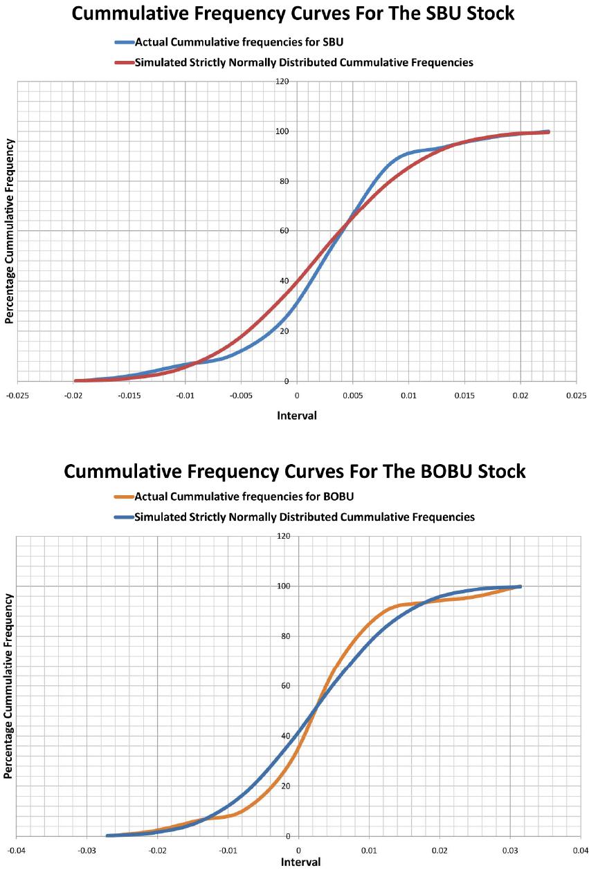

F. MAYANJA ET AL.
Open Access JMF
490
Figure 1. SBU stock.
Figure 2. BOBU stock.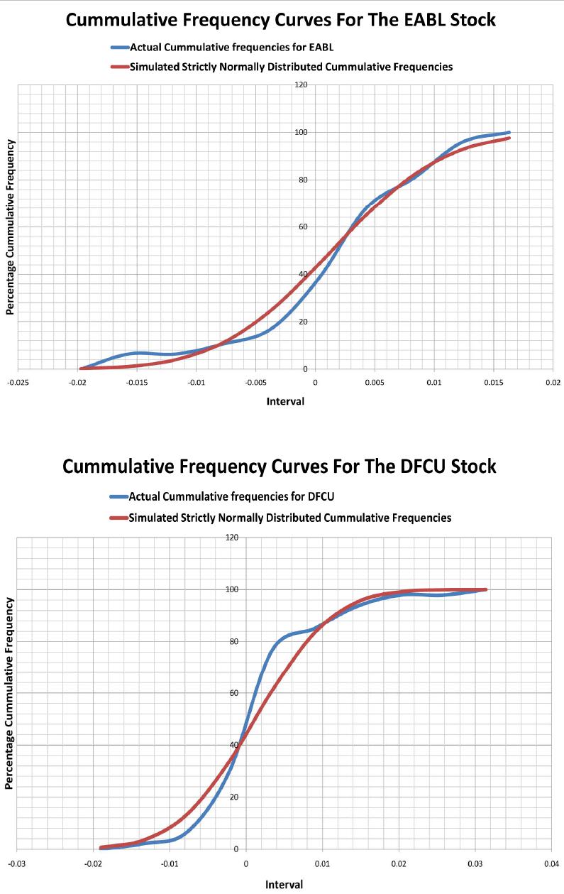

F. MAYANJA ET AL. 491
Figure 3. EABL stock.
Figure 4. DFCU stock.
Open Access JMF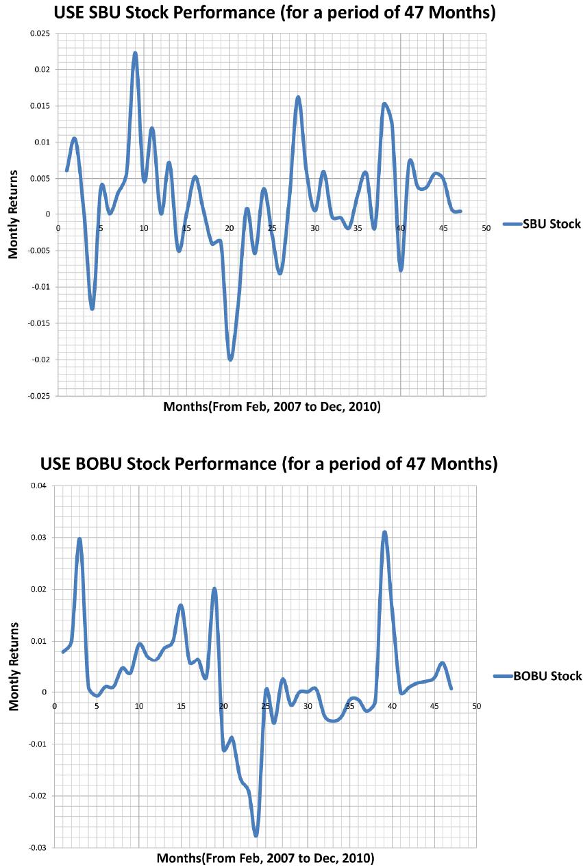

F. MAYANJA ET AL. 492
Figure 5. SBU stock performance.
Figure 6. BOBU stock performance.
Open Access JMF

F. MAYANJA ET AL. 493
Figure 7. EABl stock performance.
Figure 8. DFCU stock performance.
Open Access JMF

F. MAYANJA ET AL.
Open Access JMF
494
choosing the proportions (weights) of various assets
available. Therefore the model can be written as:
11
1
Minimize 2
nn
ij ij
ij
X
X 


1
Subject to n
ii p
i
X





1
and 1
n
i
i
X



That is, given the target expected rate of return of the
portfolio
p

, find the portfolio strategy that minimizes
the portfolio variance in returns 2
p

.
5. The Solution Method for the n-Asset
Model
First, we note that it is more convenient and easier to use
vector and matrix notation , so we formulate this model in
matrix notation;
1
Minimize , .
2
, =1
T
nT T
p
zXVXst
SXRX Xe 

 
(5.1)
where , is column vector of port-
folio weights for each security.

T
12
,,,
n
XXXX

R
V is the covariance matrix of the returns.

T
1,1,,1 ,n ee
p

is the desired level of expected return for the port-
folio.
Note that in this model formulation;
1) The admissible set includes short selling, i.e.
portfolio positions with negative weights are
allowed.

<0
i
X
2) The parameter
p

is exogenously given.
3) The model (5.1) is a convex quadratic programming
problem (i.e., the objective function is quadratic, with
linear constraints and the feasibility set S is convex).
4) The solution(s) of the program depend(s) on the
parameter
p

.
To avoid degeneracies we impose the following tech-
nical conditions:


.i All first and second moments of
the random variables exist.


.ii The vectors ,e

are linearly independent. That
is, no two securities can have the same expected return
. We note that this is typically the case
when u sing real data.



,
ij
ij


.iii The covariance matrix is strictly positive
definite. The positivity of the covariance matrix means
that all the assets are indeed risky, and this is the case
of our portfolio since we considering stocks only.
n
To illustrate why we require to be strictly positive
definite, suppose;
V

T
0 . 0 00,0,,0
T
XstXVX 
Then there exists a portfolio whose return T
p
X


has zero variance. This implies that 0p

, essentially,
that this portfolio is risk less. But, this contradicts the
idea that our portfolio consists of only risky assets. At
this stage, before we attempt to solve our formulated
problem there is need to see whether the problem has
been well formulated. That is whether a unique solution
exists.
Proposition 1.
Model problem (5.1) is a convex quadratic problem
with a unique convex solution.
Proof.
The function T
X
VX defines a quadratic form. The
matrix is symmetric and positive definite (from
condition
V


iii ), this means that is strictly convex.
The constraints are linear, which guarantees that is a
convex solution space. Moreover condition implies
that the gradients of the constraints are linearly indepen-
dent, which guarantees a unique solution. Therefore, if
conditions
zS

ii






and iiiiii hold, the model problem
(5.1) has a unique solution and hence well formulated.
6. Solution to the Formulated Model
We therefore can proceed to determine the solution, first
we note that model problem (5.1) is a constrained
classical optimization problem, with equality constraints.
It can therefore be solved by the Lagrangian method. The
La- grangean function1 for the model is


12
1
,1
2
TT T

p
LXXVX XeX




2 nPropositio (
If conditions hold, the solution to the
above problem is2; )( ))(iiiandiii


*1
12
12
22
,
with and ,
p
XV e
cba b
ac bac b





p




(6.1)
where
11
, , .
TT T
aeVebeV cV
1



 

Note that 1

and 2

depend on
p

, which is the
target portfolio mean prescribed in the variance minimi-
zation problem. The variables can be deter-
mined since and , aab nd c V

are known.
1Definition 6.1

 
. Let ,

F
LXf XgX   The function
L
is
called the Lagrangian function and the parameters

are the
L
agrange multipliers, where the functions 
and
f
XgX
are twice
continuously differentiable.
2For a thorough and detailed proof refer to pages 26-28 [1].

F. MAYANJA ET AL. 495
Hence

*1
12
XV e





can be solved. Where

T
****
12
,,,
n
XXXX
is the optimal portfolio weights. For , Equation
(6.1) bec omes; 6n
*1112131415161
1
*21 2223 2425262
2
*31 3233343536
31
*41 4243 444546
4
*51 5253545556
5
*61 6263 646566
6
1
1
1
1
1
1
aaa aaa
X
aaaaaa
X
aaaaaa
X
aaaaaa
X
aaaaaa
X
aaa aaa
X




 

 

 

 

 

 

 

 


 


32
4
5
6

























The variance3 for the optimal portfolio

2
*
p



*
X
is given by
2
2
*2
pp
p
ab
d



c .
The resulting frontiers of the un constrained problem
above for the Lagrange method is as shown in Figure 9
with the global minimum variance portfolio marked red
on the frontier4.
However this is ideal as there are restrictions in the
USE market for example no short selling, and there is a
specified sum to be invested in a particular stock there-
fore we incorporate restrictions
7. Effect of Incorporating Restrictions to the
Model
Imposing the restriction; ,,n aXbabXR , where
in general we assume that
11
1, 1
nn
ij
ij
ab




hold.
Note that 11
n
i
ia 

 is necessary for the portfolio
optimization problem to have a solution and 1
assures us that total wealth available will be invested. 1
n
j
jb 

Our optimization problem (5.1) would therefore be:


1
Minimize ,. , 1, ,,
2
TnTT
rr pn
Z
XVXstSXRXXea X babXR  

To be specific we require that the weights are non-
negative, therefore, we shall restrict

0X0a

, So we have 0
X
b

. Our problem therefore is:


1
Minimize ,. ,1, 0, , 0, ,
2
TnTT
rr pn
Z
XVXstSX RXXeXXbbX R   (7.1)
Next, we now seek to write our model as a quadratic
programming problem. First we recall that a quadratic
programming problem has the general form:

Minimize Maximize T
Z
CXX DX
Subject to , 0AXb X

T
12
,,,
n

X
xx x

T
12
,,,
n
Cccc

T
12
,,,
m
bbb b
11 1
1
n
mm
aa
A
aa







n
11 1
1
n
nn
dd
D
dd








The function T
X
VX defines a quadratic form, the
matrix is symmetric and positive, the constraints are
linear which guarantees a convex solution space. The
solution to this problem is based on the Karush-Kuhn-
Tucker (KKT) conditions5. Applying the KKT conditions
to the model problem above for we which we seek a
solution becomes6;
V

12 0
TT
ab
XV eI 
T

 
I
XSb

 1
T
XeT
p
X


n



5Historically, w. Karush was the first to develop the KKT conditions in
1939 as part of his M.S. thesis at the University of Chicago. The same
conditions were developed independently in 1951 by W Kuhn and A.
Tucker. The KKT conditions provide the most unifying theory for all
non linear programming problems [19].
6For the explicit mathematical gymnastics please refer to pages 40-42 o
f
[1].
3A reader is advised to refer to pages 29-30 of [1] for the proof.
4For a detailed proof of how the global minimum variance portfolio is
determined plea s e refer to pages 30-32 o f [1].
Open Access JMF

F. MAYANJA ET AL. 496
Figure 9. The unconstrained frontier (lagrange method).
0
3,4, ,22,
3,4, ,2,1,2, ,
kj
ai bj
XS
kn nn
jni
 
 


 n
, , , 0
ab
XS

 
And according to the theorem we must con-
sider at most different cases to find the optimal solu-
tion. It is therefore very evident at this stage, what impact
the weight restrictions have had on the solution proce-
dure. This system unlike the unrestricted model we had
before, cannot be solved analytically for assets.
Therefore we have to seek numerical algorithms to deter-
mine the optimal solution. However, the good news is
that with the current computer advancements we do not
have to struggle with the algorithms. Powerful algori-
thms for numerical methods have been developed in va-
rious softwares. For this particular problem we shall use
the excel solver , which uses the Newton Raph-
son algorithm to find the optimal solutions numerically.
These optimal portfolio returns were plotted against the
optimal standard deviation and the resulting frontier is as
shown in Figure 10.
KKT
3n
2n
2007
In an attempt to make a comparative analysis of the
effect of restriction on the level of returns we plotted
both frontiers on the same graph as shown in Figure
11.
From the graph notice that the unconstrained frontier
is superior to the constrained frontier. That is, for every
risk level, the unconstrained frontier gives a higher or
equal return as compared to the constrained frontier.
Which is as expected, since constraints or restrictions on
investment have a negative affect on the level of returns.
This is in line with the theoretical findings [20].
8. Diversification under a Portfolio with
Averagely Correlated Assets
In consideration of diversification constraint 4., we try to
explore Mathematically the effect of increasing or reduc-
ing the number of stocks held in a portfolio on the fron-
tier. That is, we shall examine the necessary and su- ffi-
cient conditions for a security to improve the Marko-
witz hyperbola (frontier).
Let


012
,,,
n
PSS S be a set of n securities
among which we may choose for our portfolio. Addi-
tionally, let




101211
\,,,,,,
iii
PPS SS SSS


n
.
Also, let
p

and q

be the Markowitz hyperbolas
for security sets and respectively.
0
P1 P
Proposition 3.
Unique portfolio weights can be determined for secu-
rities that lie on the hyperbola as a linear function of the
portfolio expected return,
p

. That is, *
p
X
gh

 ,
where g and h are known constants for a particular
portfolio.
Proof.
Recall that we have


*1
12
XV e




Open Access JMF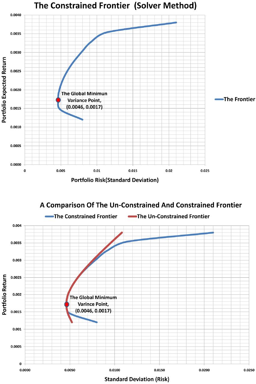

F. MAYANJA ET AL. 497
Figure 10. The constrained frontier.
Figure 11. The unconstrained and constrained frontiers.
Open Access JMF

F. MAYANJA ET AL. 498
for the un-restricted model problem. Where; Proof of (iii).
If , the linear function *
p
X
gh


1
p
cb
d



 , and 2p
ab
d




Substituting for 12 ,

 gives;

*1 pp
cbab
XV e
dd










*1 pp
ce be ab
XV d

 
 


11 11
*pp
cV e bVeaVbV
Xd

 
 
 




11 11
*pp
cV ebVaVbVe
Xdd

 





111 1
*
p
cV ebVaVbV e
Xdd


 


Therefore,


11
ha VbVe
d
*
11
,
1
where ,
1
p
Xgh
gcVebV
d







 (8.1)
T heorem 8.1 Consider equationthe above *
p
X
gh

 ,
then; , then1) If 0
ii
gh
p
q


.
0, the2) Id nf 0h an
i i
g
p
q

 and any
point on
p

has a fixe the
security.
3) If, then
non-zerod weight ofth i
0
i
h
p
q

, so
p

and q

are
tangent at e one
Proof of (i).
Assume . Then
p
xactlypoint.
0
ii
gh
0,
iiip
Xgh

 .
Hence, the security has a zero weight for every
point on
th
i
p

, an
s
ut, up
ft wi
d so it may be disregarded from
portfolio cideration as it does not improve the
hyperbola.on removing the security from
, we are leth . That is, the set of securities that
ize
on
B
q
th i
0
P
optim 1
P

. Ther, efore
p
q


.
Proof of nd , the expression p
(ii).
If 0
i
h a 0
i
giii
X
gh


0
i
h

will have
exactly one root at
*
p
g
h


.
Therefore,
*i
pi
g
h



such that will be the only
p

0
iiip
Xgh



; that is, *
p

0
i
h

if will be the only value of
p

at
whe Markyperbolas ich thowitz h
p

and q

intrsect.
use e That is beca
*i
pi
g
h


, 0
iiip
Xgh

 .
Therefore, 0
i
X

, so thesecurity is not invol-
ved.
But,
th i
and q

cannot cross each other so
p

p

is
inside o r onq

.
bo
Therefore, the intersection ofo
Marklas must be a tangent po
since
the tw
int. Also, owitz hyper
p

and q

only intersect at one point, it is clear
that
p
q


.
Corollary 1.
0
ii p
gh iffq


.
Proof.
Suppose 0
ii
gh

 does not hold. That is,


.0
i
ah

and 0
i
g

, or , (in part

.0
i
bh


.b i
g
is not conditioned because if 0
i
h whether 0
i
g

or
equals gip

 and thus, any point on
p

has a fixed
security. Recall that points non-ht o
on zero weigf the th
i
p

have
fer to Prop os
uniolios asso
(re d that each
que po
ition 1) artf
nciated with them point on
p

has
conclude that a nsecurityon-zero weight of the th i , we
p
q

.
0
i
g

the effect of the th i security car
Mathematical implication on pries the same

).
From )( iiart 0 , if and ptheorem i h0
i
g

, then
p
q


contra.a. Also
.)( iiiptheorem if 0
i
h
which
art dicts

, from

, then
p
q

 which
contradicts


.b. Therefore, we conclude that
p
q


implies 0
ii
gh

. But, from


. partithe, if
0
ii
gh orem

, then
p
q


. He,
0
enc
ii p
gh iffq



.
8.2 Theorem


11
0 0
ii
gh iffVeV 


ii

 
Proof.
Assume 0
ii
gh

, then from Equation (8.1) we have;




111 1
and
ii ii
cV ebVaVbV e 
 

From

 
11
e bV 


ii
cV
we have:
Open Access JMF

F. MAYANJA ET AL. 499
Proof.
From Corollary 1 have; if
 
11
ii
Ve V
c
b


 (8.2)
and from



11
ii
aVbVe 


we have:
 
1
Ve 1
ii
aV
b


 (8.3)
Combining Equations (8.2) and (8.3) we get;
 
2
1
ab
11 1
iii i
b
VVaV V
bc c


 
 (8.4)
In Equation (8.4) above we see that if


10
i
V 


,
then we conclude
2
b
ac
which implies 2
ac b, and that 20acb , which
is impossible!(ref
,
the proore we
proved that ). So
Since

d
f of 1claim , whe

10
i
V 
.
er to2
dacb

e b
>0
11
cV

V
ii


 , b which
im ut

10V


i
plies that also,

1
i
cV e
0

. But >0c
 
11
therefore,
,

V

10
i
e
. Hence

0 if 0ghVe V 
ii ii
 .
Conversely
Assume
 
11
0e V 

 .

ii
V
Then clearly
 

11
10
ii
cV ebV
d


 .
But recall


11
10
iii
gcVebV
d


. So, 0
i
g


.
Also,
 

11
10
aVb e 

.
But recall

ii
V
d


1V bVe
. S
11
iii
ha
d



o,.
wh plies
y 2
0
i
h
Thus,
 
11
0
ii
Ve V 


ich im
Corolla 0
ii
gh.
r

11
0 pq
ii
VV eiff



 
0
ii
gh
p
q


.
Aorem we havlso, from the2e;


11
0 0
ii ii
ghiff VeV 



.
re, Corollary 1 and Theorem together im-
ply;
Therefo 2




11
0 pq
ii
VV eiff



 .
And, Corollary 2 s the final result t we have been
seeking to prove. Corollary 2 provides a necessary and
n for some security, , to improve
a Markowitz hyperbola.
This will be so provided the add
hat
sufficient conditio1n S
ition of the 1n S

to

12 n
PS S
ich
,,,S
h
the existing security set (portfolio)
is
includes
such that the new covariance matrix new V, w
1n
S

, is invertible and the condition ;


11
11
0
new new
nn
VVe 




do when es not hold. If one wonders how this is so;


11
11
0
new new
nn
Ve 


V



does not hold, Corollary 2 imies that thenpl
p
q


.
saw that But, from proo
when f of we

1 .theorempart iii
p
q



, these two have onlyngent point
and therefore one of the two hyperbogreater than
the other. Andol
one
las i
ta
s
in this case it is the hyperba of th
poo which an extra seas been add
iginal one.
Howevere stocks in our portfolio have a
random relationship, we preferred to use the condition
we proved in Corollary 2 of chapter , which is
in the correlation of the assets; the condition
on us to compute the new covaance matrix
, that includes the additional stock anden check if
e
rtfolio tcurity hed that
is greater than the or
, since th
3
ri
th
dependent of
ly required
new
V

 
11
0
new new
VVe 



does not hold, if and when this condition does not hold
then the new stock added will improve thfrontier. We
started with a portfolio of three stocks namely; DFCU,
BU with covariance matrix, then we
added a new stock UCL and computed t cova-
riance matrix and , checcondition
and found that
e
OBU and SB V
he new
he
4new
V
;
14new
Vked t




11
44
0
new new
VVe 


,
we further added a fifth stock EABL and an computed
the new covariance matrix and which
inw EABL stock,
gai
5new
V
we got
15new
V
cluded the ne

 
11
55new new
VVe 

0


and otting the three frontiers together on the same
grobserved that the frontier for the portfolio of
upon pl
aph, we
Open Access JMF

F. MAYANJA ET AL.
Open Access JMF
500
stocks was above that of the stockhich in turn was
above that of stocks, as show Figure 12.
r conditionor diversification as derived
in Corollary 2 is valid and applicable for
the USE (restricted) model. Hence, an invesr can still
reduce portfolio risk even when his/her portfolio is made
upks only. Therefore, even for investors who are
lele for tto reduc
eaer of stock in a port-
folio.
9.
study, we have identified that the USE stock
market as a whole is stochastic, as there are no particular
months where all stocks returns are low or high, and each
st
s ha
r all correlation coefficient
5 4
n ins w
3
Therefore ou f
in chapter 3, to
of stoc
ss risk averse, it is still possibhem e
portfolio risk by incrsing the nu mb
Conclusions
In this
ock behaves randomly. This is seen from the graphs
showing individual stocks performance—Figures 5-8, in
which case we concluded that the stockve a random
relationship as their ove

;
0.15 0.3


We have also noted that the "BATU
volatile stock among them all but, still thest profi-
table amo sample of the 6 stocks.
" stock is the
mo
ng a
We have proved that the log returns ofe USE stocks
are normally distributed, which implies their returns
We have also discussed in detail the Mthematics and
theoretical advancements behind the classical MPT-mo-
agai USE
the data analysis
results agree with the theory. First, we ve showed that
the plot of stocks returns against their sdard deviation
hg
magreement
wd
Finally, we found out that the solution of the unres-
m is superior (for every level of risk,
ot newor
va
del and tested these argumentsnst the stocks
data for which we have found out that
ha
tan
(risk) is a hyperbola for both the unrestricted and the
restricted optimization model problem. Secondly, we
ave also noted that increasinthe number of stocks in
the portfolio iproves th e frontier, which is in
ith the MPT-model theory. However, since our port-
folio assets ha a random relationship we could not rely
on Markowitz’s idea. So we have provided a condition
that each extra additional stock should satisfy so as to
improve the frontier. In other words, it is not necessarily
true that every additional stock improves a frontier. It
will only do so as long as Corollary 2 condition is satis-
fied.
tricted model proble
the unrestricted frontier gives an equal or higher level of
returns as compared to the restricted frontier of the same
portfolio) to that of the restricted model problem, this as
seen from Figure 11, in which the two frontiers were
plotted together.
Though the Mathematics involved is tedious and at
times complex in general, the users of these models do
ned to ry because with th e current computer ad-
most
th
at th
have a log normal distribution. ncements a number of softwares have been developed
ready to use with out bothering about the Mathematics.
a
. Figure 12. Diversification based on corollary 2

F. MAYANJA ET AL. 501
10. Recommendations
We recommend the use of computer programmes as they
help to enhance the performance of the optimization soft-
ware and also automate the various calculations that
ould other wise be performed manually in spreadsheets. w
We also, recommend financial institutions and any other
investors who use investment models to always examine,
test and adapt these models to their investment en-
vironment before applying or using them to make in-
vestment decisions, since most of these models have
underlying assumptions which have diverse implications
mathematically, financially and economically for diffe-
rent investment environment.
In the study of the effect of imposing certain restric-
tions we focused mainly on the mathematical implica-
tions. We therefore, recommend that further research
should be done on the economic and financial im-
plications of the modifications or restrictions like re-
stricting the weights with in particular bounds, number of
stocks held in a portfolio, cost constraints, ad ministrative
and policy restrictions on the MPT-model in the context
of the USE investment environment. A more realistic
model that incorporates such factors as: brokerage costs
(commissions), the Uganda Capital Markets Authority
(CMA) regulatory constraints, taxes, inflationary rates,
central depository costs and foreign exchange move-
ments (as there are cross listings in the USE market)
needs to be developed so as to reflect the true picture of
the USE trading env ironment.
Finally, there is need to revisit the
lassical MPT-
environment. Such modi-
CAPM (which was
model), so as a direct consequence of the c
to modify it to suite the USE
fications can start from the most obvious issues like co-
rrecting the beta )(

estimations of the various com-
panies in the USE (as there is a common mistake of
assuming 1=

) for most companies, to more in depth
mathematical analysis b ehind the CAPM so as to adapt it
to the USE environ ment. This is very important since the
CAPM is used in the valuation of capital assets in the
investment sector in Uganda to date.
REFERENCES
[1] M. Fredrick, M. Sure and M. Charles, “Portfolio Optimi-
Budgets,” The Review of Economics and Statistics, Vol.
47, No. 1, 1965, pp. 13-39.
[6] W. F. Sharpe, “Capital Asset Prices: A Theory of Market
Equilibrium under Conditions of Risk,” Journal of Fi-
nance, Vol. 19, No. 3, 1964, pp. 425-442.
[7] P. Krokhmal and S. Uryasev, “Portfolio Optimization
with Conditional Value-at-Risk Objective and Constraints
Center for Applied Optimization,” University of Florida,
Gainesville, 2001, pp. 32611-6595.
[8] S. Uryasev, “Portfolio Optimization with Conditional
Value-at-Risk Objective and Constraints Center for Ap-
plied Optimization,” University of Florida, Gainesville,
1999, p. 32611.
[9] Y. Kroll, H. Levy and H. M. Markowitz, “Mean-Variance
versus Direct Utility Maximization,” The Journal of Fi-
nance, Vol. 39, No. 1, 1984, pp. 47-62.
[10] H. Konno and H. Yamazaki, “Mean-Absolute Deviation
Portfolio Optimization Model and Its Applications to
Toky o Stoc k Mark et Mana geme nt, ” Science, Vol. 37, No.
5, 1991, pp. 519-531.
[11] T. Kariya, “Distribution of Stock Prices in the Stock
Market of Japan,” Toyo Keizai Publishing Co., Tokyo,
1989.
[12] G. Arnold, “Corporate Financial Management,” 3rd Edi-
tion, Pearson Education Limited, 2008.
[13] Uganda Securities Exchange, “Frequently Asked Ques-
s about USE,” 2010. www.use.or.ug
No. 4, 1974, pp. 1265-1274.
zation Model: The Case of Uganda Securities Exchange,”
LAP LAMBERT Academic Publishing GmbH & Co. KG,
Ltd., Saarbrücken, 2012.
[2] A. V. Puelz, “A Stochastic Convergence Model for Port-
folio Selection,” Operations Research, Vol. 50, No. 3,
2002, pp. 462-476.
[3] H. M. Markowitz, “Portfolio Selection,” The Journal of
Finance, Vol. 7, No. 1, 1952, pp. 77-91.
[14] A. B. Mayanja and K. Legesi, “Cost of Equity Capital
and Risk on USE: Equity Finance; Bank Finance, Which
One Is Cheaper?” MPRA Paper No. 6407, Economic
Policy Research Centre, First Brokerage House, Wash-
ington DC, 2007.
[15] E. J. Elton and M. J. Gruber, “Portfolio Theory When
Investment Relatives Are Log normally Distributed,”
Journal of Finance, Vol. 29,
[4] H. M. Markowitz, “Portfolio Selection: Efficient Diversi-
fication of Investments,” John Wiley & Sons, New York,
1959.
[5] J. Lintner, “The Valuation of Risk Assets and the Selec-
tion of Risky Investments in Stock Portfolios and Capital
tions and Answer
http://dx.doi.org/10.1111/j.1540-6261.1974.tb03103.x
[16] H.-S. Lau, “On Estimating Skewness in Stock Returns
Management,” Science, Vol. 35, No. 9, 1989, pp. 1139-
1142. http://dx.doi.org/10.1287/mnsc.35.9.1139
[17] D. J. Wheeler and D. S. Chambers, “Introduction to Skew-
ness and Kurtosis,” SPC Press, Inc., Knoxville, 1992.
[18] S.-P. Wan, “Modern Portfolio Theory Bussiness 442:
Investments,” Chapter 5, 2000.
[19] A. T. Hamdy, “Newblock Operations Research an Intro-
duction,” 8th Edition, Pearson Education, Inc., University
of Arkansas, Fayetteville, 2007.
[20] M. Jackson and M. Staunton, “Advanced Modelling in
Finance Using Excel and & Sons, Ltd.,
Chichester, 20 VBA,” John Wiley 01.
Open Access JMF