Advances in Pure Mathematics, 2013, 3, 647-652
Published Online November 2013 (http://www.scirp.org/journal/apm)
http://dx.doi.org/10.4236/apm.2013.38086
Open Access APM
The Behavior of Normality when Iteratively Finding the
Normal to a Line in an lp Geometry
Joshua M. Fitzhugh, David L. Farnsworth
School of Mathematical Sciences, Rochester Institute of Technology, Rochester, USA
Received October 20, 2013; revised November 20, 2013; accepted November 27, 2013
Copyright © 2013 Joshua M. Fitzhugh, David L. Farnsworth. This is an open access article distributed under the Creative Commons
Attribution License, which permits unrestricted use, distribution, and reproduction in any medium, provided the original work is
properly cited.
ABSTRACT
The normal direction to the normal direction to a line in Minkowski geometries generally does not give the original line.
We show that in lp geometries with repeatedly finding the normal line through the origin gives sequences of
lines that monotonically approach specific lines of symmetry of the unit circle. Which lines of symmetry that are ap-
proached depends upon the value of p and the slope of the initial line.
1p
Keywords: Minkowski Geometry; Geometric Construction; Iteration; Normality; lp Geometry; Radon Curve
1. Introduction
Minkowski geometries are completely characterized by
their unit circle, which is centrally symmetric about the
origin and convex [1: p. 17]. The spaces are homogene-
ous (all points are the same) and generally anisotropic
(the yard stick for distance is not the same in all direc-
tions). Our principal interest is the planar Minkowski lp
geometries with . Their unit circles are
1p
1
p
p
xy. (1)
The exponent p must be at least 1 in order for the unit
circle to be convex. Convexity is required for the triangle
inequality [1: pp. 22,23]. If , this is Euclidean
geometry. If , the circle is not strictly convex. As
discussed in Section 2, since in Minkowski geometries a
necessary and sufficient condition for uniqueness of
normal directions to lines is that the unit circle be strictly
convex, we do not consider the case. Convex unit
circles are strictly convex if they contain no line seg-
ments. The l1 geometry is well studied and is sometimes
called taxicab, Manhattan, or city-block geometry [2].
Since the unit circle for the limiting case is the
square with vertices , we do not consider that
geometry, as well. Figure 1 shows some lp unit circles
and the circle with , which does not produce a
Minkowski geometry since the circle is not convex.
2p
1p

1p
p

1, 1
0.5p
The unit circle determines distances. For the Min-
kowski distance between points P1 and P2, consider line
L through the origin O and parallel to the line through P1
and P2. The distance between P1 and P2 is the quotient of
0.8
1.6
-0.8
00.8 -0.8
y
-1.6
-1.6 1.6
x
Figure 1. Unit circles =1
pp
x+y for p = 0.5, 1, 1.5, 2, 4
and 6. The circles with p = 1, 1.5, 2, 4 and 6 give Minkowski
geometries.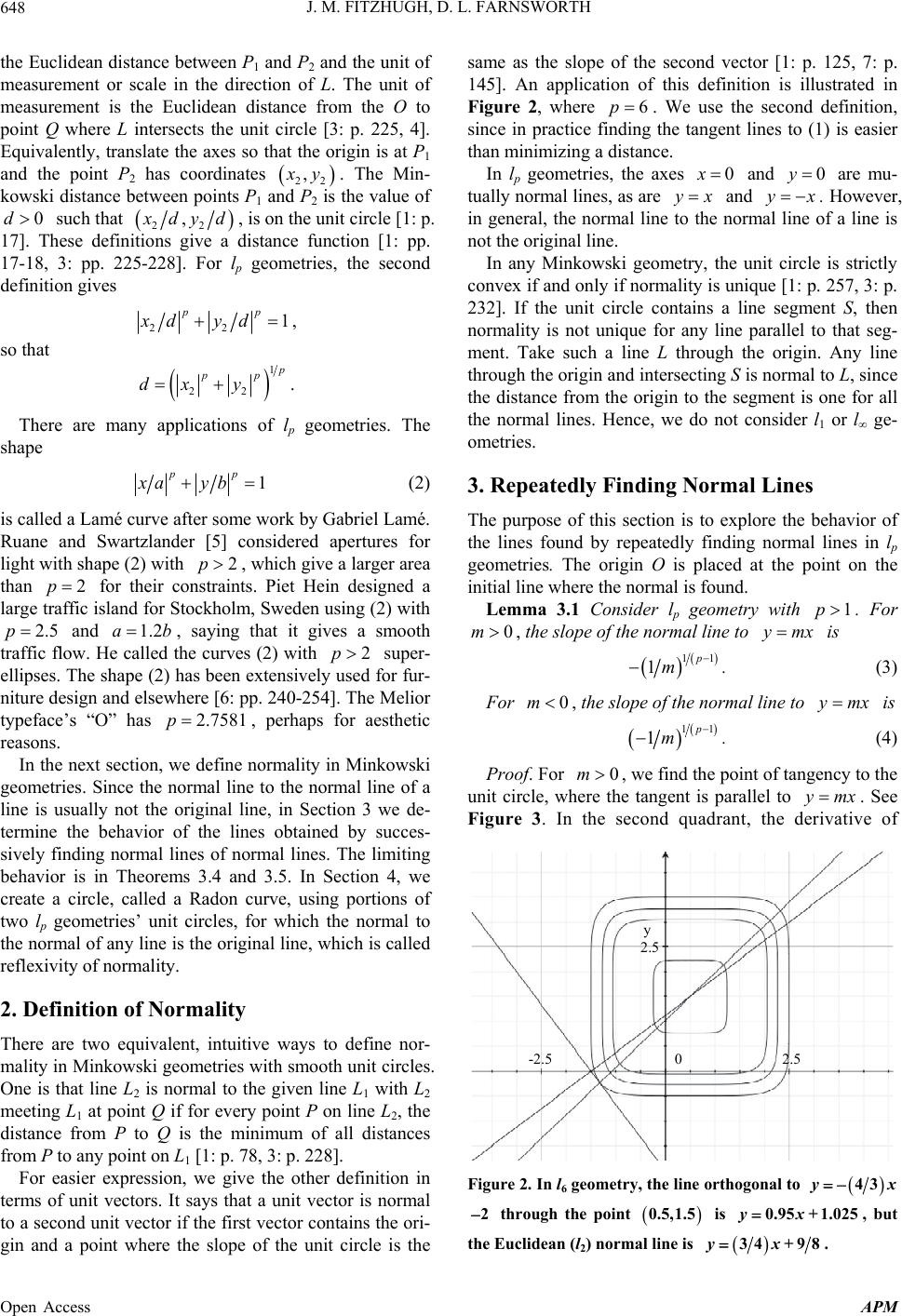

J. M. FITZHUGH, D. L. FARNSWORTH 648
the Euclidean distance between P1 and P2 and the unit of
measurement or scale in the direction of L. The unit of
measurement is the Euclidean distance from the O to
point Q where L intersects the unit circle [3: p. 225, 4].
Equivalently, translate the axes so that the origin is at P1
and the point P2 has coordinates

22
,

x
y. The Min-
kowski distance between points P1 and P2 is the value of
such that 0d

22
,
x
dy d, is on the unit circle [1: p.
17]. These definitions give a distance function [1: pp.
17-18, 3: pp. 225-228]. For lp geometries, the second
definition gives
22
1
pp
xd yd,
so that

1
22
p
pp
dx y .
There are many applications of lp geometries. The
shape
pp
xa yb1
b
(2)
is called a Lamé curve after some work by Gabriel Lamé.
Ruane and Swartzlander [5] considered apertures for
light with shape (2) with , which give a larger area
than for their constraints. Piet Hein designed a
large traffic island for Stockholm, Sweden using (2) with
and , saying that it gives a smooth
traffic flow. He called the curves (2) with super-
ellipses. The shape (2) has been extensively used for fur-
niture design and elsewhere [6: pp. 240-254]. The Melior
typeface’s “O” has , perhaps for aesthetic
reasons.
2p
2.7581
2p
2.5p1.2a
p
2p

In the next section, we define normality in Minkowski
geometries. Since the normal line to the normal line of a
line is usually not the original line, in Section 3 we de-
termine the behavior of the lines obtained by succes-
sively finding normal lines of normal lines. The limiting
behavior is in Theorems 3.4 and 3.5. In Section 4, we
create a circle, called a Radon curve, using portions of
two lp geometries’ unit circles, for which the normal to
the normal of any line is the original line, which is called
reflexivity of normality.
2. Definition of Normality
There are two equivalent, intuitive ways to define nor-
mality in Minkowski geometries with smooth unit circles.
One is that line L2 is normal to the given line L1 with L2
meeting L1 at point Q if for every point P on line L2, the
distance from P to Q is the minimum of all distances
from P to any point on L1 [1: p. 78, 3: p. 228].
For easier expression, we give the other definition in
terms of unit vectors. It says that a unit vector is normal
to a second unit vector if the first vector contains the ori-
gin and a point where the slope of the unit circle is the
same as the slope of the second vector [1: p. 125, 7: p.
145]. An application of this definition is illustrated in
Figure 2, where 6p

. We use the second definition,
since in practice finding the tangent lines to (1) is easier
than minimizing a distance.
In lp geometries, the axes and are mu-
tually normal lines, as are and . However,
in general, the normal line to the normal line of a line is
not the original line.
0x
yx
0y
yx
In any Minkowski geometry, the unit circle is strictly
convex if and only if normality is unique [1: p. 257, 3: p.
232]. If the unit circle contains a line segment S, then
normality is not unique for any line parallel to that seg-
ment. Take such a line L through the origin. Any line
through the origin and intersecting S is normal to L, since
the distance from the origin to the segment is one for all
the normal lines. Hence, we do not consider l1 or l ge-
ometries.
3. Repeatedly Finding Normal Lines
The purpose of this section is to explore the behavior of
the lines found by repeatedly finding normal lines in l
p
geometries. The origin O is placed at the point on the
initial line where the normal is found.
Lemma 3.1 Consider lp geometry with . For
, the slope of the normal line to is
1p
mx0my


11
1p m . (3)
For 0m

, the slope of the normal line to ymx

is


11
1p m . (4)
Proof. For , we find the point of tangency to the
unit circle, where the tangent is parallel to
0m
ymx

. See
Figure 3. In the second quadrant, the derivative of
0 -2.52.5
2.5
y
Figure 2. In l6 geometry, the line orthogonal to


43yx
2

through the point


0.5,1.5 is , but
the Euclidean (l2) normal line is
0.95 +1.025yx


34 +98yx.
Open Access APM

J. M. FITZHUGH, D. L. FARNSWORTH 649
0 0.8 -0.8 -1.6 1.6
0.8
-0.8
-1.6
1.6
y
y
= mx
P
x
Figure 3. OP is normal to=
y
mx .

1
p
p
xy gives

1
dd
p
yx xy  . Setting this
equal to m gives


11
1p yxm  , which is the slope
of the normal line to . Formula (4) is derived
similarly. □
ymx
Lemma 3.2 Consider lp geometry with . Desig-
nate by mn the slope of the nth line found by iteratively
finding normal lines at the origin, starting with the line
with . For even n,
1p
0
ymx00m


2
11
2
p
nn
mm

, (5)
and for odd n,


2
11
2
p
nn
mm

 . (6)
For even n,


11
0
n
p
n
mm  , (7)
and for odd n,


11
0
1n
p
n
mm

 . (8)
These formulas can be appropriately altered for 00m

.
Proof. To obtain (5), for even n, using (3),


11
11p nn
mm

 (9)
and using (4) and (9),









2
11
21
11
11
11
1
11
.
p
nn
p
p
n
p
n
mm
m
m







 



Equation (5) supplies


2
11
20
p
mm   and also the
main induction step to give (7). Similarly, obtain (6) and
(8). □
Lemma 3.3 Consider lp geometry with . If
1p
0,1 0,2
1mm

, (10)
then
,1 ,2
1
n
mm
n

, (11)
where the second subscript indicates the identity of the
line.
Proof. Take m0,1 and m0,2 to be positive. The proof for
negative initial slopes is similar. For even n, using (7) for
line 1, (10), and then (7) for line 2 give




11 11
,1 0,10,2,2
11
nn
pp
nn
mmm m

 .
The proof of (11) for odd n uses (8) and (10) in a simi-
lar manner. □
Because of the symmetries of the lp unit circle about
the axes, only 0 need be considered. The condi-
tion
0m
0,1 0,2
m1m

between the slopes of two initial lines
means that the lines have the same angle with the respec-
tive axes. Lemma 3.3 shows the symmetries about
y
x

 in the behavior of the iterated normal lines, so
only initial slopes between 0 and 1 need to be considered.
Theorem 3.4 Consider lp geometry with . For
the initial line 0
2p
ymx

with 0, the subse-
quence of
0m1


n
m for even n has values and
monotonically approaches 1, and the subsequence for
odd n has values
01
n
m
1
n
m

 and monotonically ap-
proaches –1. For the initial line 0 with ,
the subsequence of
ymx0 m1


n
m
n
m
for even n has values
and monotonically approaches 1, and the subsequence
for odd n has values and monotonically ap-
proaches –1.
1
n
m
1
Proof. Take 0
0m1

. Using Lemma 3.2, for even n,


2
11
2
p
nn
mm

 n
m
and

 11
0
Limit Limit1
n
p
n
nn
mm

 

.
For odd n,


2
11
2
p
nn
mm

 n
m
and




11
0
LimitLimit1 1
n
p
n
nn
mm

 


1
.
Lemma 3.3 says that initial lines 0 with ymx
0
0m


01m
give the behavior of the iterated normal lines
for . □
Open Access APM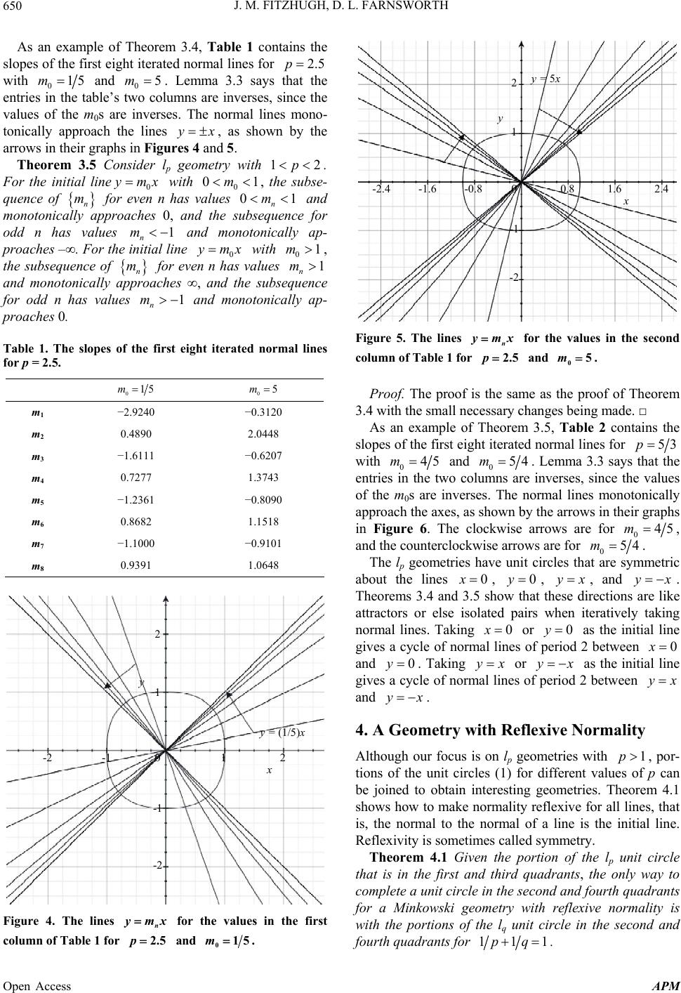

J. M. FITZHUGH, D. L. FARNSWORTH 650
As an example of Theorem 3.4, Table 1 contains the
slopes of the first eight iterated normal lines for 2.5p

with 015m and 0. Lemma 3.3 says that the
entries in the table’s two columns are inverses, since the
values of the m0s are inverses. The normal lines mono-
tonically approach the lines
5m
y
x, as shown by the
arrows in their graphs in Figures 4 and 5.
Theorem 3.5 Consider lp geometry with 12p


1
01
n
m
01m
1
n
m
.
For the initial line0 with 0 0, the subse-
quence of for even n has values and
monotonically approaches 0, and the subsequence for
odd n has values and monotonically ap-
proaches –∞. For the initial line 0 with ,
the subsequence of for even n has values
and monotonically approaches , and the subsequence
for odd n has values and monotonically ap-
proaches 0.
ymx
n
m

n
m
n
m
m
ymx

n
m
1
1
Table 1. The slopes of the first eight iterated normal lines
for p = 2.5.
015m 05m
m1 −2.9240 −0.3120
m2 0.4890 2.0448
m3 −1.6111 −0.6207
m4 0.7277 1.3743
m5 −1.2361 −0.8090
m6 0.8682 1.1518
m7 −1.1000 −0.9101
m8 0.9391 1.0648
0 1 -1 -2 2
x
-1
-2
1
2
y
y = (1/5 ) x
Figure 4. The lines n
y
mx
2.5p
for the values in the first
column of Table 1 for and 015m.
0 0.8 -0.8-1.61.6 2.4-2.4
x
y
-1
-2
1
2 y = 5x
Figure 5. The lines n
y
mx
2.5p
for the values in the second
column of Table 1 for

and .
05m
Proof. The proof is the same as the proof of Theorem
3.4 with the small necessary changes being made. □
As an example of Theorem 3.5, Table 2 contains the
slopes of the first eight iterated normal lines for 53p

with 045m

and 054m

. Lemma 3.3 says that the
entries in the two columns are inverses, since the values
of the m0s are inverses. The normal lines monotonically
approach the axes, as shown by the arrows in their graphs
in Figure 6. The clockwise arrows are for 045m

,
and the counterclockwise arrows are for 054m.
The lp geometries have unit circles that are symmetric
about the lines 0x

, , , and 0yyxyx

.
Theorems 3.4 and 3.5 show that these directions are like
attractors or else isolated pairs when iteratively taking
normal lines. Taking 0x

or as the initial line
gives a cycle of normal lines of period 2 between
0y
0x

and 0y

. Taking yx

or as the initial line
gives a cycle of normal lines of period 2 between
yx
yx

and yx

.
4. A Geometry with Reflexive Normality
Although our focus is on lp geometries with , por-
tions of the unit circles (1) for different values of p can
be joined to obtain interesting geometries. Theorem 4.1
shows how to make normality reflexive for all lines, that
is, the normal to the normal of a line is the initial line.
Reflexivity is sometimes called symmetry.
1p
Theorem 4.1 Given the portion of the lp unit circle
that is in the first and third quadrants, the only way to
complete a unit circle in the second and fourth quadrants
for a Minkowski geometry with reflexive normality is
with the portions of the lq unit circle in the second and
fourth quadrants for 11pq 1

.
Open Access APM

J. M. FITZHUGH, D. L. FARNSWORTH 651
Table 2. The slopes of the first eight iterated normal lines
for p = 5/3.
045m 054m
m1 −1.3975 −0.7155
m2 0.6053 1.6521
m3 −2.1236 −0.4709
m4 0.3231 3.0946
m5 −5.4439 −0.1837
m6 0.0787 12.702
m7 −45.269 −0.0221
m8 0.0033 304.58
0 1 -1 -2 2
x
y
-1
1
2
y = (4/5 ) x
y = (5/4 ) x
Figure 6. The lines n
y
mx for the values in Table 2 for
53p with 045m and 054m.
Proof. Since Minkowski unit circles are symmetric
about their centers, we can reference only the first and
second quadrants. Take the center to be the origin, and
construct all normal lines at the origin. In the first quad-
rant, the unit circle is . In the second quad-
rant, the unit circle is
pp
xy1


y
gx

22
. The original line L1 is
, , which intersects at the point
111
. The construction is illustrated in Figure 7 for
p = 4. For reflexivity, demand that the slope of line L1
equals the slope of the tangent line L3 at the point
222
with
ytx

,Px

,Px
0t

y

y
pp
xy1
y
gx
xy
, and demand that the slope
of the line L2 tangent to at 1
pp



111
,Pxy
equals the slope 22 xy of the line L4, which is to be
orthogonal to line L1. The goal is to find the function

g
x. The slope of L2 is found by taking the derivative
of to obtain
pp
xy1
11
dd0
pp
pxpyy x

.
Then,
  
1
111
dd 1
p
p
p
p
yx xyxtxtt


 .
Equating the slopes of the lines L1 and L3 gives
02
P
2
P
1
L
1
L
3
L
2
L
4
y
2.5
.5
Figure 7. The unit circle in this Minkowski geometry is
44
+=xy1
in quadrants 1 and 3 and
43 43
+=xy1 in
quadrants 2 and 4. Li nes L1 and L3 are parallel, as are lines
L2 and L4. In this geometry, normality is reflexive, that is, L4
is normal to L1 and L1 is normal to L4 for any choice of L1.

2
ddtyxx (12)
with


y
gx. Equating the slopes of lines L2 and L4
gives
1
22
p
ty

x. (13)
Solving (13) for t gives


11
22
p
tyx

 . (14)
Equating the expressions for t in (12) and (14) and
dropping the subscript 2 give the differential equation






111 1
11
dd or dd
pp
p
yxyxyyxx



 ,
whose unique solution is



1
1pp pp
yx

C

 .
Since




00yg1

, . Designating 1C


1pp

by q gives 11pq 1

 and
1
qq
xy


for


y
gx in the second and fourth quadrants. □
The unit circles 44
1xy

 and 43431xy


are dual, since




14 1431

. Dual unit circles and
dual spaces are central to Minkowski geometry [1,3,7].
Schäffer’s theorem says that dual unit circles have the
same circumferences, when the circumferences are mea-
sured with their own distance functions [1: pp. 111-118,
Open Access APM

J. M. FITZHUGH, D. L. FARNSWORTH
Open Access APM
652
7: p. 153, 8,9]. Because of the symmetry of the unit circle
in Theorem 4.1, it has the same circumference as the dual
lp and lq unit circles whose arcs compose it.
Radon curves are equivalently defined as either unit
circles for which normality is reflexive for all lines or
unit circles that have arcs of dual circles in alternating
quadrants as in Theorem 4.1’s example [1: p. 128, 3: pp.
233-234, 7: pp. 143-145, 10].
REFERENCES
[1] A. C. Thompson, “Minkowski Geometry,” Cambridge
University Press, Cambridge, 1996.
http://dx.doi.org/10.1017/CBO9781107325845
[2] E. F. Krause, “Taxicab Geometry,” Dover Publications,
New York, 1986.
[3] R. V. Benson, “Euclidean Geometry and Convexity,” Mc-
Graw-Hill, New York, 1966.
[4] B. V. Dekster, “An Angle in Minkowski Space,” Journal
of Geometry, Vol. 80, No. 1, 2004, pp. 31-47.
[5] G. J. Ruane and G. A. Swartzlander Jr., “Optical Vortex
Coronagraphy with an Elliptical Aperture,” Applied Op-
tics, Vol. 52, No. 2, 2013, pp. 171-176.
http://dx.doi.org/10.1364/AO.52.000171
[6] M. Gardner, “Mathematical Carnival,” Alfred A. Knopf,
New York, 1975.
[7] J. C. Álvarez Paiva and A. Thompson, “On the Perimeter
and Area of the Unit Disc,” The American Mathematical
Monthly, Vol. 112, No. 2, 2005, pp. 141-154.
http://dx.doi.org/10.2307/30037412
[8] J. J. Schäffer, “The Self-Circumferences of Polar Convex
Disks,” Archiv de Mathematik, Vol. 24, 1973, pp. 87-90.
http://dx.doi.org/10.1007/BF01228179
[9] J. B. Keller and R. Vakil, “p, the Value of  in lp,” The
American Mathematical Monthly, Vol. 116, No. 10, 2009,
pp. 931-935.
http://dx.doi.org/10.4169/000298909X477069
[10] J. Radon, “Über eine Besondere Art Ebener Konvexer
Kurven,” Berichte der Sächsische Akademie der Wissen-
schaften zu Leipzig, Vol. 68, 1916, pp. 131-134.