Journal of Water Resource and Protection
Vol. 3 No. 2 (2011) , Article ID: 4056 , 6 pages DOI:10.4236/jwarp.2011.32013
Modelling Open Channel Flows with Vegetation Using a Three-Dimensional Model
1Key Laboratory of Pollution Processes and Environmental Criteria (Ministry of Education), College of Environmental Science and Engineering, Nankai University, Tianjin, China
2Cardiff School of Engineering, Cardiff University, The Parade, Cardiff, UK
3State Key Hydroscience and Engineering Laboratory, Tsinghua University, Beijing, China
E-mail: gaogh@nankai.edu.cn, FalconerRA@cf.ac.uk, LinBL@cf.ac.uk
Received December 6, 2010; revised January 7, 2011; accepted February 10, 2011
Keywords: hydrodynamic, turbulence model, vegetation
ABSTRACT
The effects of vegetation on the flow structure are investigated in this paper. In previous studies of modelling vegetated flows, two-equation turbulence models, such as the  model, were often used. However, this approach involves a level of uncertainty since the empirical coefficients in these two equations have not yet been satisfactorily obtained for such flow conditions. In addition to this, two extra partial differential equations needing which will result in an increase in the computational cost. The main purpose of the study was therefore to try and acquire accurate velocity profiles without the more advanced two-equation turbulence models. A three-dimensional model using a simple two layer mixing length model was therefore used. The governing hydrodynamic equations were refined to include the effects of drag force induced by vegetation on the flow structure. The model was applied to an experiment flume to study the flow field with vegetations, where experiment data are available. Distributions predicted by the model were compared with laboratory measured ones, with very good agreements being obtained. The results showed that the simple mixing length model could produce accurate complex velocity profile predictions requiring fewer coefficient data and less computation.
1. Introduction
Vegetation has become central to river and coastal restoration schemes, the creation of flood retention space and coastal protection project [1]. The existence of vegetation within the watercourse tends to increase the hydraulic resistance by dragging and turbulence [2]. The mixing induced by the turbulence will have significant effect on the pollutant and sediment transport processes in the water. [3] The structure of vegetated open channel flows is three-dimensional and highly complicated. Wilson and Shaw [4] proposed the modified  turbulence model, which was based on the assumption that the drag force produces additional turbulent energy in the flow and increases the dissipation rate. However, this method introduced two weighting coefficients, which need to be calibrated for each study. For practical projects such calibration is not desirable [1,5,6]. Fischer-Antze et al. [7] used the standard
  model to predict both submerged and emergent vegetation flows, with satisfactory results being obtained. However, considerable computational efforts were required for a 3-D model simulation, particularly due to the needs to solve two extra partial differential equations.
The main purpose of the study presented in this paper was therefore to try and acquire accurate three-dimensional velocity profiles without the need for more advanced two-equation turbulence models. A simple two layer mixing length model was refined to take into account the effects of drag force induced by vegetation on the flow structure, with the refinement being included in a three-dimensional hydrodynamic model. Vegetated open-channel flows have been classified into three types, depending upon the relative height of vegetation  to the total water depth
![]() , namely terrestrial canopy flows
, namely terrestrial canopy flows , flows with submerged vegetation
  and flows with emergent vegetation [8-10]. The terrestrial canopy flows are similar to the flows over very rough beds, so this kind of flows can be treated by introducing additional flow resistance. Therefore, the terrestrial canopy flows are not considered in this study. The concentration is focused on the submerged and emergent vegetated flows.
2. Numerical Model
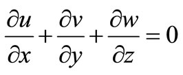
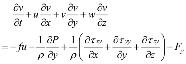
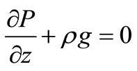
To model the effects of the vegetation on flow structure, the three-dimensional layer integrated numerical model was refined to include the drag force induced by the vegetation on the flow structure. The model solves the Reynolds averaged Navier-Stokes equations under the hydrostatic pressure assumption, which is written as:
 (1)
(1)
 (2)
(2)
 (3)
(3)
 (4)
(4)
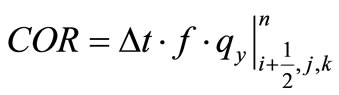
where t = time, x, y and z = Cartesian co-ordinates in the horizontal (x, y) and vertical (z) directions; u, v, w = components of velocity in the x, y, and z direction, respectively; P = pressure,  = density of water;
  = Coriolis parameter; g = gravidity acceleration;
  = vegetation induced drag force in the x, y directions respectively, which is included as sink terms in the momentum equation.
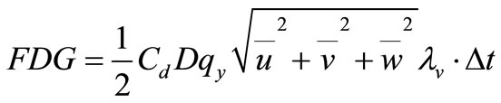
The drag force induced for per unit height of a rigid rod per unit area can be expressed as:
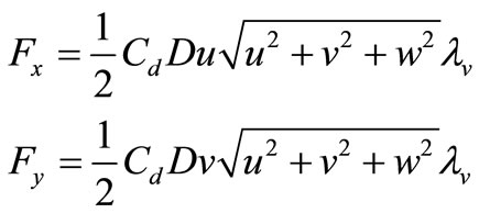 (5)
(5)
where  drag coefficient, which is typically 1.2 for a circular cylinder;
 ![]() diameter of the respective vegetation stem;
diameter of the respective vegetation stem;  vegetation density.
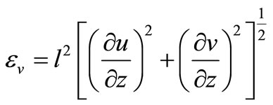
Many researches [7] have used the  turbulence closure to simulate the effect of vegetation on the flow structure, with reasonable agreement being obtained between experiment data and model predictions. In order to acquire accurate velocity profiles without the need for more advanced two-equation turbulence models, which requires values for many unknown coefficients, a simple two layer mixing length model was therefore refined and included in the three-dimensional model. The vertical eddy viscosity was represented using a two layer mixing length model as proposed by Rodi [11]:
 (6)
(6)
where l is the mixing length, defined as :
 for
for 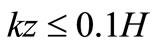
 for
for 
and k is von Karman’s constant.
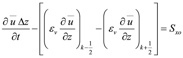
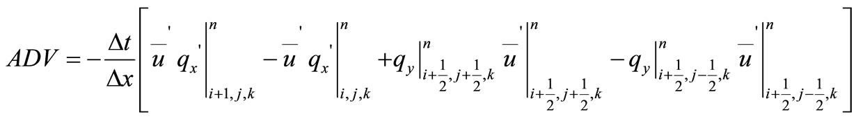
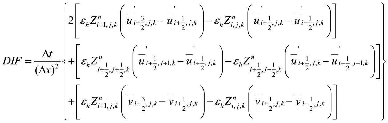
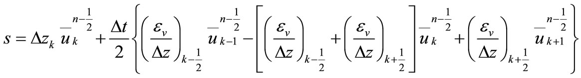
Equations (1)-(4) were solved using the finite difference scheme on a rectangular mesh in horizontal, and a layer integrated finite difference scheme on a irregular mesh in the vertical [12]. Figure 1 shows the locations of the key variables defined for the three-dimensional finite difference mesh in the vertical plane. The layer integrated governing equations are solved using a combined explicit and implicit scheme. The vertical diffusion terms were treated implicitly, whilst the remaining terms were treated explicitly.
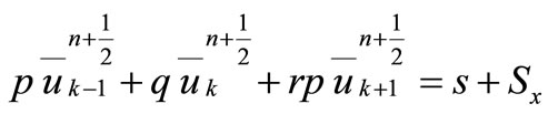
For the first half time step the depth integrated equations are solved to obtain the water elevation field across the domain. The layer integrated equations in the x direction are solved using the water elevation obtained from solving the depth integrated equations. Lin and Falconer [12] expressed the momentum equation in the x direction as follows:
 (7)
(7)
where  represents the terms treated explicitly. The following is the finite difference representation for equation:

Figure 1. Vertical grid system.

 (8)
(8)
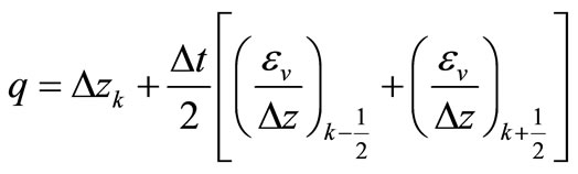
where
 (9)
(9)
and

Re-arranging Equation (8) gives:
 (10)
(10)
where:
 ,
,  ,
,  ,
,
where  velocity component in x direction at
 layer. Equation (10) can be expressed in a matrix form for the different layers, where
  for the surface and
  for the bottom layer:
Thomas algorithm has been used to solve this tri-diagonal matrix to obtain the velocity in the x direction. Once the water elevations and velocity component in the x direction have been solved, then the vertical velocity ![]() can be determined for each layer across the computational domain using the continuity equation.
can be determined for each layer across the computational domain using the continuity equation.
3. Laboratory Experiment Study
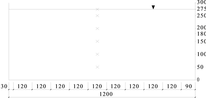
The experiment study of vegetated open channel was conducted by Dorcheh [13]. Three sets of experimental data, including: no-vegetation, submerged vegetation and emergent vegetation tests were chosen from data collected in a wide rectangular open channel flume. The flume had a width of 1200 mm and a maximum depth of 300 mm. For the vegetated flow conditions, both emergent and submerged vegetation tests were considered for three vegetation densities, namely: low density, medium density and high density. In this study only the low density vegetation data were used to test the numerical model.
In these experiments rigid wood rods were used to represent the vegetation. The rods used in Dorcheh [13] were 24 mm in diameter and 180 mm in length for the submerged conditions and 300 mm in length for the emergent conditions. The flow rate was kept a constant for all of these experiments and velocity measurements were taken at two cross-sections. The cross-sections were located at the mid-length along the flume, i.e. at 4.4 m, and near the end of the channel, i.e. at 1.4 m from the outlet. In the vertical direction measurements were taken at 50 mm from the channel bed and at 50mm intervals towards the water surface, i.e. at 50, 100, 150, 200, 250 and 275 mm. Figure 2 shows the layout of the crosssections and the measuring points for different experiment conditions. The distance between the rods in the flow direction was uniform at 0.208 m.
4. Model Application
This refined model was used to predict the structure of vegetated open channel flow. The model results were compared with the measured data obtained from the experiments mentioned above. The model was used to three open channel cases: no-vegetation, submerged vegetation and emergent vegetation flows.
4.1. Non-Vegetated Open Channel Flow
Numerical simulations for the case without vegetation were carried out first. The predicted velocity distributions along the vertical direction were compared with the measured data at the 1.4 m and 4.4 m cross-sections. The measurement locations are shown in Figure 2 and the comparisons of the results are shown in Figure 3. It can be seen that good agreement has been obtained between the measured and computed results.
 (a)
(a) (b)
(b)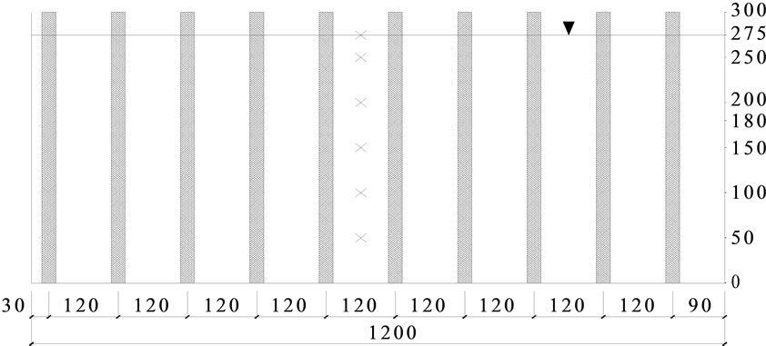 (c)
(c)
Figure 2. Layout of cross-section and measuring points for (a) no vegetation, (b) submerged vegetation and (c) emergent vegetation.
4.2. Submerged Vegetation Open Channel Flow
The numerical model was then set up to study the submerged vegetation case. Model predicted velocity distributions in the vertical direction were compared with the measured data at the 1.4 m and 4.4 m cross-section, respectively, and along the central line of the flume. The comparisons are shown in Figure 4. Again good agreement has been obtained between the measured and predicted velocity distributions. It can be seen from Figure 4 that the existence of vegetation causes a decrease in the magnitude of the velocities (or total flow component) in the vegetation layer, whereas the flow velocity or flow increases in the non-vegetated layer. The reason for that is the vegetation resistance produce a velocity defect at the vegetated region and the continuity requirement redirects the flow to the region above the vegetation [3]. The sharp velocity gradient at the top of the vegetated layer

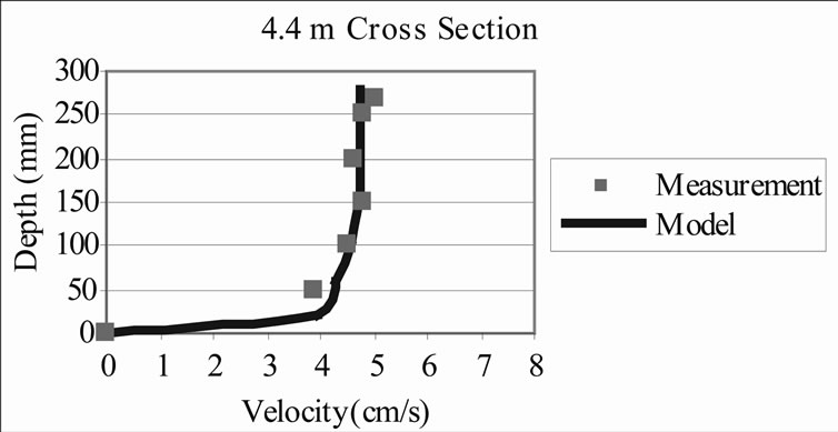
Figure 3. Velocity profile comparisons at 1.4 m and 4.4 m cross-sections for non-vegetated flows.
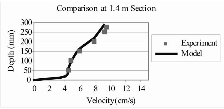

Figure 4. Velocity profile comparisons at 1.4 m and 4.4 m cross-sections for submerged vegetation flow.
will generate strong turbulence. The velocity profile can be divided in to three layers: low vegetated layer, upper-non-vegetated layer and transition layer. From Figure 4 it can be seen that the sharp velocity gradient were formed at near the bottom of the vegetation and near the top of the vegetation. The sharp gradient near the bed was formed due to the effect of the bed friction and the sharp gradient near the top of vegetation due to the drag force exerted by vegetation, which will form a shear layer.
4.3. Emergent Vegetation Open Channel Flow
Figure 5 shows comparisons of the model predicted vertical velocity distributions against experiment data for flow through emergent vegetation. Again it can be seen that the results are encouraging, particularly for the relatively simple mixing length model used. The velocity distributions over an emergent vegetation layer are nearly uniform, but close to the bed the velocity increases rapidly form the zero. It shows that the velocity near the bottom is control by both the bed roughness and the vegetation drag, the uniformity show that the velocity distribution affect mainly by the vegetation drag force.
5. Conclusions
Details are given of the refinement of an existing three-dimensional model to include the drag force introduced by vegetation in the momentum equation. A simple two layer mixing length turbulence closer is used in this model. The model was applied to a physical model channel, to investigate the effects of vegetation on the flow structure. Model predicted velocity distributions were compared with laboratory data measured, with very good agreements being obtained for all three sets of experiments. The results showed that the simple two layer mixing length model could produce accurate complex velocity profile predictions, with the advantage of requiring less calibration coefficients than some of the commonly used higher order models.

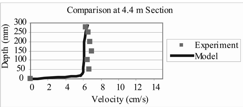
Figure 5. Velocity profile comparisons at 1.4 m and 4.4 m cross-sections for emergent vegetation flow.
6. Acknowledgements
The authors would like to acknowledge the support of this project from Environment Agency and European Regional Development Fund. The first author was supported by “the Fundamental Research Funds for the Central Universities”.
REFERENCES
- C. A. M. E. Wilson, T. Stoesser and P. D. Bates, “Modelling of Open Channel through Vegetation,” In: P. D. Bates, S. N. Lane and R. I. Ferguson, Eds., Computational Fluid Dynamics: Applications in Environmental Hydraulics, John Wiley & Sons Ltd., 2005. doi:10.1002/0470015195.ch15
- S. Choi and H. Kang, “Numerical Investigations of Mean Flow and Turbulence Structures of Partly-Vegetated Open-Channel Flows Using the Reynolds Stress Model,” Journal of Hydraulic Research, Vol. 44, No. 3, 2006, pp. 203-217. doi:10.1080/00221686.2006.9521676
- C. W. Li and K. Yan, “Numerical Investigation of WaveCurrent-Vegetation Interaction,” Journal of Hydraulic Engineering, Vol. 33, No. 7, 2007, pp. 794-803. doi:10.1061/(ASCE)0733-9429(2007)133:7(794)
- N. R. Wilson and R. H. Shaw, “A Higher Order Closure Model for Canopy Flow,” Journal of Applied Meteology, Vol. 16, No. 11, 1977, pp. 1198-1205. doi:10.1175/1520-0450(1977)016<1197:AHOCMF>2.0.CO;2
- F. Lopez and M. Garcia, “Open Channel Flow through Simulated Vegetation: Turbulence Modelling and Sediment Transport,” Hydrosystems Laboratory, Department of Civil Engineering, University of Illinois, 1997.
- T. Tsujimoto, Y. Shimizu, T. Kitamura and T. Okada, “Turbulent Open Channel Flow over Bed Covered by Rigid Vegetation,” Journal of Hydroscience and Hydraulic Enigineering, Vol. 10, No. 2, 1992, pp. 13-25.
- T. Fischer-Antze, T. Stoesser, P. Bates and N. R. B. Olsen, “3D Numerical Modelling of Open Channel Flow with Submerged Vegetation,” Journal of Hydraulich Research, Vol. 39, No. 3, 2001, pp. 303-310. doi:10.1080/00221680109499833
- S. Choi and W. Yang, “CFD Modelling Vegetated Channel Flows: A State-Of-Art Review,” Water Engineering Research, Vol. 6, No. 3, 2005, pp. 101-112.
- A. Murota, T. Fukuhara and M. Sato, “Turbulence Structure in Vegetated Open Channel Flows,” Journal of Hydrologic and Hydraulic Engineering, Vol. 2, No. 1, 1984, pp. 47-61.
- H. M. Nepf and E. R. Vivoni, “Flow Structure in DepthLimited Vegetated Flow,” Journal of Geophysical Research, Vol. 105, No. 12, 2000, pp. 547-557. doi:10.1029/2000JC900145
- W. Rodi, “Turbulence Models and Their Application in Hydraulics,” 2nd Edition, International Association for Hydraulics Research, Delft, the Netherlands, 2000, pp. 104.
- B. Lin and R. A. Falconer, “Three-Dimensional Layerintegrated Modelling of Estuarine Flows with Flooding and Drying,” Journal of Estuarine, Coastal and Shelf Science, Vol. 44, No. 6, 1997, pp. 737-751. doi:10.1006/ecss.1996.0158
- S. A. M. Dorcheh, Effect of Rigid Vegetation on the Velocity, Turbulence and Wave Structure in Open Channel Flows, PhD Thesis, Cardiff University, 2007.