Technology and Investment
Vol.2 No.2(2011), Article ID:5167,19 pages DOI:10.4236/ti.2011.22011
Assessing Uncertainty and Risk in Public Sector Investment Projects
Macquarie University, Sydney, Australia
E-mail: stefan.trueck@mq.edu.au
Received March 4, 2011; revised April 13, 2011; accepted April 16, 2011
Keywords: Risk Analysis Techniques, Monte Carlo Simulation, International Financing Institutions
Abstract
The feasibility and profitability of large investment projects are frequently subject to a partially or even fully undeterminable future, encompassing uncertainty and various types of risk. We investigate significant issues in the field of project appraisal techniques, including risks and uncertainties, appropriate risk analysis, project duration as well as the dependencies between (sub-) projects. The most common project appraisal techniques are examined addressing benefits and weaknesses of each technique. Furthermore, the practical use of the different techniques for the public sector is examined, exemplifying this with a small-scale analysis of the risk analysis procedures of the World Bank. Our findings suggest that in particular for the public sector, practical implementation of quantitative techniques like Monte Carlo simulation in the appraisal procedure of investment projects has not fully occurred to date. We strongly recommend further application of these approaches to the evaluation of processes and financial or economic risk factors in project appraisal of public sector institutions.
1. Introduction
Assessing the feasibility and profitability of large investment projects requires the consideration of various aspects and procedures. The projected outcomes of feasibility and profitability are frequently subject to a partially or even fully undeterminable future, encompassing uncertainty and various types of risk. With current investment markets evolving within an increasingly volatile and highly interlinked global network, investment projects are intensely exposed to uncertainties surrounding costs, completion time and the extent to which the original objectives of the project can eventually be achieved.
In undertaking procedures for analysing the risk and uncertainty surrounding a project, the potential outcome of project feasibility and profitability can be assessed. In addition, it is often possible to identify ways in which the project can be made more robust, and to ensure that residual risks are well managed. Investment appraisal procedures are generally carried out by applying cost-benefit analysis and/or risk analysis tools. Usually, cost-benefit analysis (excluding the process of risk analysis) focuses only on either the mean or mode of the net present value (NPV) or internal rate of return (IRR) [1]. There are many methods for analysing the effects changes in factors have on the NPV (or any other output variable of interest). Well known and widely applied techniques include break-even analysis, sensitivity analysis, scenario analysis, risk analysis, decision trees and uncertainty analysis [2].
A review of literature and evaluation reports reveals a common scenario that the assessment of such values does not provide enough information for a valid decision; particularly for public sector investment projects in highly uncertain environments such as developing countries. Risk analysis is not a substitute for standard investment appraisal methodology but rather a tool for enhancement of results. Although risk and uncertainty analysis has evolved to become a valid component in the project appraisal process for both private and public investment projects, different extents of practical implementation remain [3]. Such analysis supports the investing organization in its decision by providing a measure of the variance associated with a project appraisal return estimate. By being in essence a decision-making tool, risk analysis has many applications and functions that extend its usefulness beyond purely investment appraisal decisions.
Given this variety of applications, different models and appraisal techniques are employed in praxis, generating a diverse landscape of investment appraisal procedures. The application of techniques and models generally utilised within the private sector is well covered in the literature, whereas their implementation in the public sector lacks sufficient review to date. Parson et al. [4] and Lempert [5] point out the diversity of public organizations’ objectives and interests. They argue that this could be seen as a reason for scenario analysis methods usually aiming at small groups may not be applicable for large public organizations. On the one hand, Little and Mirrlees [6] and Devarajan et al. [7] argue that quantitative risk analysis has experienced great alterations over the last decades. While in the 1980s the practical implementation of in-dept quantitative risk analysis methods was dismissed in favour of sensitivity analysis [8,9], in the 1990s its practical use within project appraisals was reinstated [10-12]. In the last decade, due to increasing computational power and availability of statistical software, quantitative analysis and techniques have become even more popular. However, Fao and Howard [13] argue that many public organizations (including government departments) have institutionalised scenario-planning exercises to anticipate the impact of risks and the estimation of future trends of external influences instead of using for example Monte Carlo Simulation. On the other hand, in the light of evolving economic concerns the use of investment appraisal using Monte Carlo techniques has become increasingly important in the practical world [14]. Monte Carlo methods can be used to compute the distributions of project outcomes, initiated with prior information about the distributions of variables which determine the discounted return of a project. A complete distributional mapping provides not only the expected return, but additionally an evaluation of the risk and a distribution of alternative outcomes what could be considered as a huge advantage for project appraisal also for public sector institutions.
This paper aims to address the possibility of practical implementation for the various project evaluation techniques applied within both the private and public sector. Hereby, a special emphasis is set on the use of Monte Carlo Simulation and practical implementation of risk analysis techniques within the public sector. We present a review of the literature on project appraisal techniques in the presence of risk and uncertainty. The first part outlines given problems and issues in the field of project appraisal techniques, including risks and uncertainties, appropriate risk analysis, issues regarding duration as well as the dependencies between (sub-) projects. The most common project appraisal techniques are examined and benefits and weaknesses of each technique will be addressed. Furthermore, we analyse the practical use of different techniques for the public sector, exemplifying this with a small-scale analysis of the risk analysis procedures of the World Bank (WB).
2. Problems and Issues
2.1. Risks and Uncertainties: How can They be Treated?
Risks and uncertainties frequently have a decisive impact on the course and the outcome of projects. The outcomes of some events possess the continuing feature of constricted foreseeability or even entire unpredictability. Recent developments show that due to several features including advanced technology, more sophisticated modelling approaches and in-depth informative sources, the possibilities of accurate predictions within risk analysis have been enhanced. The performance of the accuracy of these predictions depends on the complexity of the system, in which the risk variable is embedded, as well as on the quality of available input information and the extent of its associated potential errors, most commonly deriving from data, modelling or forecasting [15].
Despite the crucial importance of risks and uncertainties on an investment project’s performance, both terms are often used interchangeably in practice. As shown below, the available literature demonstrates that there has been an extensive and controversial debate on the possibility and scope to differentiate between these two terms.
Risk and uncertainty were initially differentiated in Knight’s study Risk, Uncertainty and Profit [16]. Knight distinguished between the two terms by stating that risks encompass events for which outcomes are known or are quantifiable due to historical evidence and probability distributions. This implies the feature that in a risky situation an insurable outcome is given, which has further been interpreted by Weston [17] and Stigler [18]. Another differentiation, based on Knight’s theory of profit, is the assumption that in such a risky outcome profit cannot exist. This is underlined by the assumption that if all countermeasures to reduce or even eliminate risks are utilised, then Knight considers all outcomes to be certain and risk free. Furthermore, his differentiation describes uncertain events where it is not possible to specify numerical probabilities, creating uninsurable outcomes [16]. Hence, as apposed to a situation of risk, Knight considers uncertainty as a condition in which profit can exist.
Knight’s determination has entailed a controversial debate ever since and many authors have denied his approach to be valid [19,20]. Despite certain critical points, the fundamentals of Knight’s distinction are thoroughly relevant for the purposes of this paper as he reviews various project appraisal techniques based on probability distributions. Based on Knight’s statements, on the one hand risk can be defined as quantifiable randomness with a historic and probable nature due to recurring events. Uncertainty on the other hand originates from an infrequent discrete event in which information on the probability distribution is lacking. As the probability of the possible outcomes is not known in the situation of uncertainty, the expected (or mean) outcome is more often used in practice. Figures 1 illustrates the specification of probability distributions in the respective situations of risk and uncertainty.
The evaluation and containment of project risk and uncertainty can be best accomplished with a successful assessment of the nature of uncertainty surrounding the key project variables. Assessing the origin, degree and potential consequences of a project’s risk and uncertainty is best undertaken by an elaborate and deliberate risk management concept, involving numerous steps for assessing each type of risk and for investigating the overall risk profile. Numerous classifications of risk types have been undertaken [21,22]. Vose [23] categorised risk classifications into the following exemplifying sections:
· Administration
· Project Acceptance
· Commercial
· Communication
· Environmental
· Political
· Quality
· Resources
· Strategic
· Subcontractor
· Technical
· Financial
· Knowledge and information
· Legal As this paper focuses on project appraisal techniques for public financial investment projects, the classification of the financial risks will be of main interest. Van Greuning and Bratanovic [24] further exemplified the types of financial risks, which are shown in Table 1.
The risk management concept implies adequate and qualitative information in order to restrain the scope of risk and uncertainty for a project’s forecast. Frequently, the information imposes a certain error quote as it is to a high degree based on expert opinion. Despite the most likely wide experience of the financial analyst and their knowledge about the source and accessibility of the information, the occurrence of an error rate is often inevitable. The nature of financial risks further endorses this complex matter, as it is e.g. difficult to forecast with exact accuracy the rate of general inflation for the following year [25].
2.2. Procedure of Risk Analysis
The process of risk management for projects has been well defined in terms of its methodological aspects
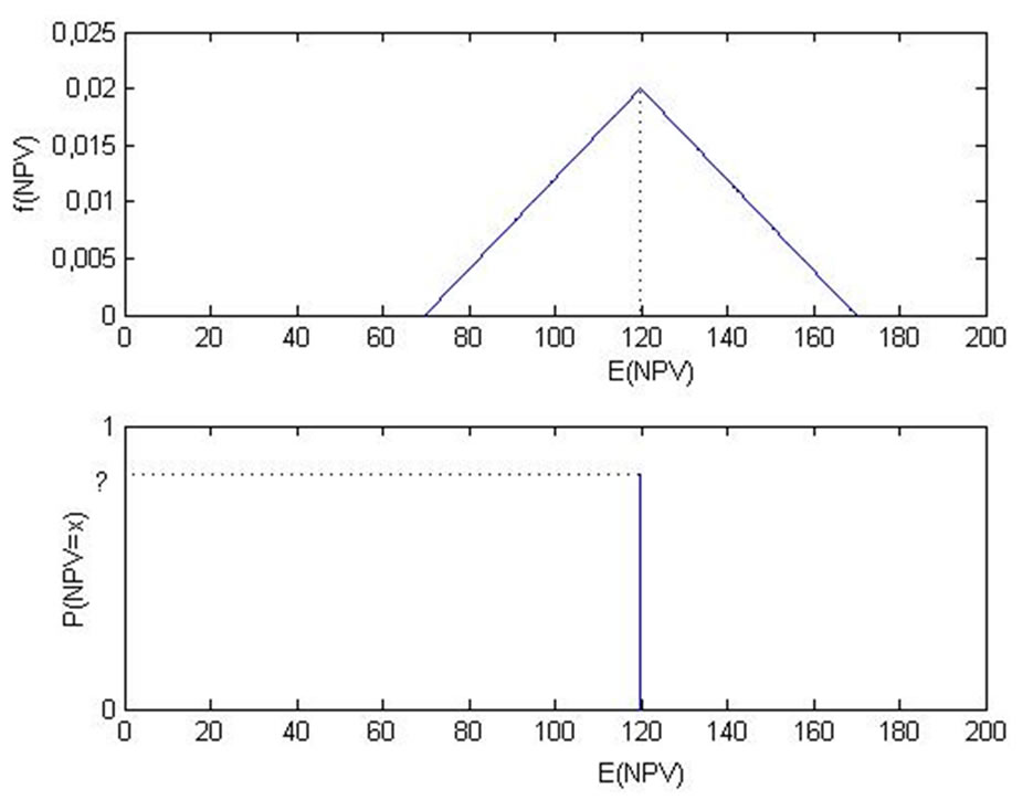
Figure 1. Illustration of the specification for probability distributions in the situations generally referred to as “Risk” (upper panel) and “Uncertainty” (lower panel). In the “Risk” case, randomness of the event can be quantified by a probability distribution. Here, e.g. a triangular distribution with expected value of 120, minimum value of 70 and maximum value of 170 is assumed. In the “Uncertainty” case information about the probability distribution is lacking such that in practice often only the expected outcome of 120 is used.
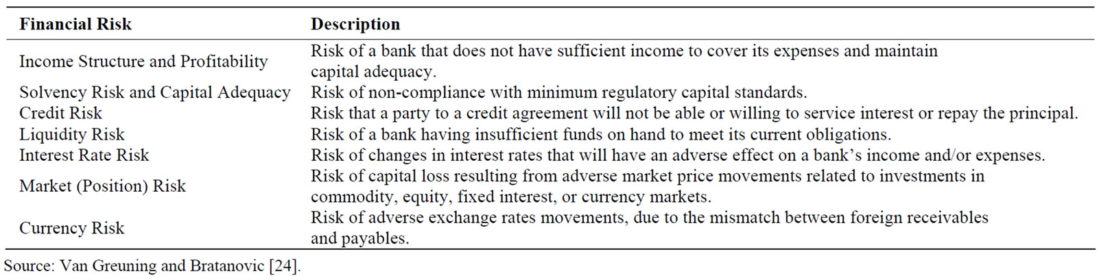
Table 1. Summary of financial risk factors.
[21,26]. One of the first attempts to define the structure of the risk management process was undertaken by Hertz and Thomas [27], in which the process was broadly set up by risk identification, measurement, evaluation and re-evaluation. Over the years, this classification has been further extended by the more continuous steps of monitoring and the consequential step of action planning [21,26]. Despite numerous attempts to structure the risk management process, in practise the dynamics of a project’s life cycle and environment and actors often demand changes and ongoing restructuring of the process [28]. Given the research aim of this paper, the process of risk analysis (more precisely quantitative risk analysis) will be the focal point within the process of risk management, as shown in Figure 2 below. The risk management process contains several steps and actors. Obviously, the figure simplifies the structure of a project risk management process by focussing on the risk analysis process and on the two acting levels of the risk manager and risk analyst. The decision-making level is in charge of determining any potential problems within the projects’ objectives, including the identification of the risk management target, an objective function and measure of performance.
After reviewing all available data, the risk analysis process is initiated by generating a forecast model which determines formulas for the project’s variables (e.g. operating costs) that have an impact on the forecast of the project’s outcome. In a second step, the risk analyst is required to define crucial risk variables. A risk variable is defined as a variable that is “critical to the viability of the project in the sense that a small deviation from its projected value is both probable and potentially damaging to the project worth” [25].
In the next step the problem of uncertainty and risk is approached by setting margins in order to provide a range of the risk variable’s values and additionally by allocating probability weights to each range. A risk analyst utilises the project’s information to quantitatively describe uncertainty and risk of the project by using probability distributions. Although this approach does not provide the analyst with an exact prediction of the value, probability distributions increase the likelihood of forecasting the actual value within the margins of an appropriately chosen range. When defining probability distributions, relationships between risk variables are often encountered, connoting a given correlation between them.
Based on the project’s risk values and derived probability distributions for the risk factors, by using simulations, a probability distribution for the project’s outcome can be determined. The application of simulation runs and run numbers depends on the employed model, which will be further illustrated in Section 3. The result of each run is calculated and gathered for the final step of statistical analysis and interpretation. Eventually, validation of the risk analysis model is required and amendments can be made where necessary. The final step of reviewing and analysing the results is frequently undertaken on a mutual basis by the decision-maker and the risk analyst.
At this point it should be mentioned that further limitations in practice are given when tackling the problem of quantification of risks and uncertainties. The information essential for such an estimation is frequently limited in terms of accessibility and transparency. These limitations are often even more pronounced within public sector institutions that require data and information not only for private sector projects but also for other public institutions [30].
2.3. Sensitivity to Factors
Investment project evaluation is embedded in a dynamic and constantly changing environment, exerting influences on the values and predictions of the risk analysis. If it is desired that all possible consequences and outcomes are taken into consideration, the effect of potential changes from the shifting environment on the project’s risk values have to be measured in advance. The aim of such an analysis is to identify if and which variables sensitively react to a great extent to external changes, eventually contributing greater uncertainty to the project
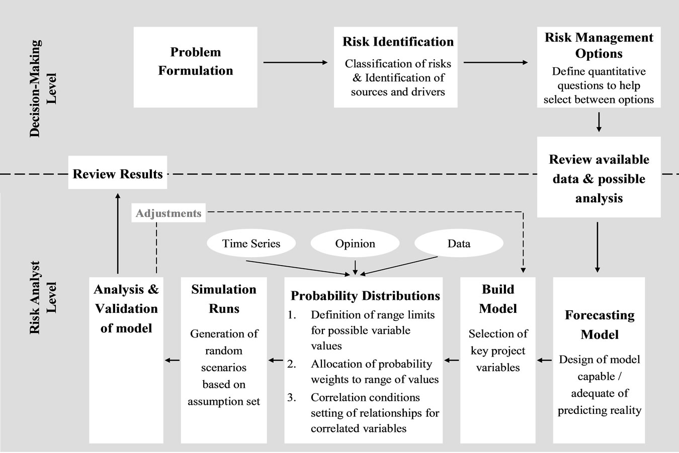
Figure 2. Description of the risk analysis process. Source: Author’s own compilation based on Savvides [25] and Vose [29].
forecast [22]. The external changes effectuate certain input values (income, costs, value of investments, etc.) to influence certain criteria values (e.g. NPV) and the overall investment project evaluation. The sensitivity of the project’s revenue (in terms of NPV, cash flows or other measurements) is quantified on the basis of all available past data of the chosen measurement for the project’s revenue as well as of the essential risk variables. NPV calculations are very sensitive to external influences such as changes in economic growth, interest rates, inflation rates or currency exchange rates. The project’s sensitivity to external effects can be measured by several other factors including i.e. the value of the project’s capital. Going beyond the sphere of a project’s sensitivity to its impact on an entire organization, Jafarizadeh and Khoshid-Doust [31] state that the value of a firm is the most suitable factor when measuring the organization’s sensitivity towards external factors. The premise for measuring this influence is that the firm is publicly traded.
The assessment of susceptibility of risk variables is undertaken in the early stages of a risk analysis procedure, most commonly at the initial stage when building the model and defining the models’ risk variables. Sensitivity analysis and uncertainty analysis in form of quantitative risk analysis should both be part of a comprehensive risk management procedure, in which uncertainty analysis is consecutively built on the results of the sensitivity analysis [32]. Estimating possible susceptibility of the models’ risk variables can also enhance project formulation and appraisal by improving the allocation of resources available for design work and further data collection.
2.4. Risk Adjustments
By using the available data, the degree of variation for the project’s risk variable can be determined by setting range limits (domain) with a minimum and a maximum value around the value that a projected variable may hold. This first step of defining the probability distribution within the risk analysis process is usually undertaken by constructing a uniform distribution, which is a comparably easy way of allocating the likelihood of risk [33]. Of course, the application of other probability distributions like e.g. the normal, triangular or also asymmetric distributions is possible. With historical data it is also possible to distribute the frequency of a risk variable. This can be undertaken by grouping the number of occurrences of each outcome at successive value intervals, expressing the frequencies in relative not absolute terms.
Another approach to determine outcome risk and uncertainty is by defining the so-called “best estimate”, where the values of the mode, mean, or a rather conservative estimate are taken [25]. However, this approach interferes with the graphical explanation of an uncertain situation as depicted in Figure 1, in which the mean is usually used. This inconsistency further underlines the interchangeable use of the terms risk and uncertainty in practise.
During the course of the risk analysis it may be necessary to undertake risk mitigation, where the ranges of the variables are either reduced or expanded. After finding a base estimate and performing a risk analysis, specified risks are then mitigated and eventually risk analysis (both sensitivity and probability analysis) is repeated. This step is required when certain identified risks have been countervailed, such as the improvement of skills of the project management. Merna and Von Storch [34] exemplified such a process in their case study of crop production in a developing country. Mitigation of some commercial risks identified in their analyses were reduced or even eliminated through measures such as insurance cover or hedging currencies.
2.5. The Optimal Scheduling of Projects/Risk Analysis
A further problem within risk management is appropriate project scheduling with project revenue being dependent on the time of realisation. Most literature addresses this issue with the project’s revenue (e.g. NPV) being independent of the time of realisation [35-37]. Recent literature has focussed more on formulating a project schedule in which revenue is dependent on project duration. Etgar et al. [38] formulated an optimisation programme for this problem; comparing their final NPVs with the NPVs of early start schedules and late start schedules for 168 different problems. Their results revealed that project revenue planning depends on the project duration, which is crucial for the optimisation of a project’s success and a less risky completion.
Another crucial step in the risk analysis is to adequately define the type of problem distribution that can be used for project task duration estimates. A risk analyst can select from a variety of probability distributions that describe the time scale of a project.
While distributions with a finite range such as the triangular distribution explicitly define a possible minimum and maximum value for the duration, distributions with an infinite range like e.g. the lognormal distribution enable the possibility to exceed the upper limit of the task duration. Note that specifying a finite range for the duration implies that any possibility of completing the task prior to the minimum duration or that the task will continue past the maximum duration limit is essentially denied. Given this condition, Graves [39] asserted that distributions with a finite range are less employable in praxis. Sometimes completely unexpected “showstopper” issues may arise and cause problems in the project. He further claims that using distributions with an infinite range, the project manager is better able to get a base estimate, a contingency amount, and an overrun probability estimate, instead of the usual most-likely, worst case and best case estimates.
Williams [40] gave a systematic description of a number of analytical approaches to project scheduling, naming the major problem of these methods to be “the restrictive assumptions that they all require, making them unusable in any practical situations”. These analytical methods often only captured certain moments of the project duration, instead of entire project duration distributions. Such distributions were more practical in defining the confidence level of project completion dates and could best be realised with the simulation runs undertaken through the Monte Carlo Method.
2.6. Dependence between Several Projects Variables
When defining and running simulations of probability distributions, certain dependencies between risk variables and those of other projects may be encountered. Both projects of the private and public sector come across independencies of their risk variables, especially when numerous projects of different sectors are analysed. However public institutions such as the World Bank have encountered difficulties when comparing project profitability and risks across sectors, since the measurement of costs and benefits differs from sector to sector and according to Baum & Tolbert [41] “indices such as the net present value and the internal rate of return are not a sound yardstick for inter-sectoral resource allocation”. Due to the extent of discussion on this subject, the focus will be set on dependencies within one project and the matter of cross-sectoral or multi-project comparison will not be further considered. Further reference hereto can be found in Florio [30].
This interactive relationship is especially expedited by external factors, making it possible that several risk variables change simultaneously. Within a risk analysis this problem is dealt with by defining the degree of correlation, where the analyst has the option to choose between techniques for approximate modelling of correlation or more sophisticated techniques.
The simplest way to correlate probability distribution is by using rank order correlation, where the distributions are correlated and the results are given on a scale between −1 and +1. If the model’s results from simulations in the case of independence and correlated risk factors are significantly different, the correlation is perceptibly an important component of the general project model. In such cases, the analyst is advised to use a more sophisticated technique such as correlation matrices or the envelope method. As the purpose of this paper is not an in-depth description of correlation analysis, further detail can be found in numerous references on risk analysis [29,42,43]. In instances where the simulation results for independent and correlated risk factors are comparably similar, it might be sufficient to undertake a rank order correlation, which is a non-parametric statistic for quantifying the correlation relationship between two variables. This situation implies no casual relationship, nor probability model. Van Groenendaal and Kleijnen [2] address the situation when several factors change simultaneously, crediting the Monte Carlo simulation for taking this issue into account.
2.7. Selection of Discount Rate
With completion of the risk analysis, the analyst obtains a series of results which are organized and presented in the form of a probability distribution of the possible outcomes of the project. Despite the advantages of picturing and interpreting the results, some interpretation issues regarding the use of the net present value criterion remain.
In praxis, distribution of NPVs generated through the application of risk analysis are often ambiguous when making an investment criteria decision. The selection of an appropriate discount rate is frequently crucial for realistic projection of a project’s performance and literature has delved into the different methods to find the appropriate discount rate.
Brealey and Myers [44] or Trigeorgis [45] suggest the risk-free interest rate to be the most appropriate discount rate used in a project appraisal subject to risk analysis, allowing no previous judgement of the risk level in a project. Conversely, in deterministic project appraisal procedures, a risk premium is usually included in the discount rate [46-48]. This risk premium is usually measured as the difference between the expected return of similar projects and the risk-free interest rate. Another school of thought maintains that the discount rate should include a premium for systematic (or market) risk but not for unsystematic (or project) risk [49-51].
Choosing the appropriate discount rate with or without a risk premium depends on the subjective conception on the predisposition towards risk. If the decision-maker is more risk-adverse, the risk premium will be relatively high and mostly projects with relatively high return will be considered for investment.
3. Project Appraisal Techniques
3.1. Expert Opinions/Scenario Analysis
3.1.1. Scenario Analysis
Scenario assessment is the basic tool implemented in assessing risk and uncertainty about future forecasts [52]. As described above, the future of projects is frequently uncertain and requires a certain degree of risk to address this state of dubiety by constructing possible scenarios in order to determine the option that performs best with minimum risk.
Principally, scenarios assess the influence of different alternatives on a project’s development. The combined consideration of certain “optimistic” and “pessimistic” values of a group of project variables facilitates to demonstrate different scenarios, within certain hypotheses. In order to define such optimistic and pessimistic scenarios it is necessary to choose for each critical variable extreme values among the range defined by the probability distribution. Project performance indicators are then calculated for each hypothesis. In this case, usually an exactly specified probability distribution is not needed.
In the process of risk analysis for investment projectshistorical data on low-frequency, high-severity events is often lacking, resulting in impediments when estimating their probability distributions. To overcome these difficulties, it is often obligatory to include scenario analysis in the model for risk quantification. As a result, scenario analysis provides rough quantitative assessment of risk frequency and severity distributions based on expert opinions. Decision-making for such less risky outcomes may be done on the basis of selecting the scenario that possesses the most benefit with minimum risks and impacts.
Since scenario analysis originated in the 1970s, it has become a common decision-making tool among financial and insurance companies especially within asset-liability and corporate risk management. A vast range of literature on the issue has been compiled to this end, of which a key thematic selection is presented in this paper. For a review and classification of scenario analysis techniques see e.g. Von Notten et al. [53] or Bradfield et al. [54]. In the last four decades, eight general categories (types) of scenario techniques with two or three variations per type have been developed, resulting in numerous techniques overall. The most commonly utilised technique is the qualitative approach of the Royal Dutch Shell/Global Business Network (GBN) matrix, created by Pierre Wack in the 1970s and popularised by Schwartz [55] and Van der Heijden [56]. The GBN matrix is based on two dimensions of uncertainty or polarities. The four cells of the matrix symbolise four mutually exclusive scenarios. Each of these four scenarios is then elaborated into a complete account in order to discuss implications for the focal issue or decision.
As this paper’s objective is not to focus on a complete evaluation of all discussed scenario analysis techniques, it shall refer in-depth only to the below-mentioned references at this point.
The review of Börjeson et al. [57] typology categorises three different futures (what will happen; what can happen; and how a specific target can be achieved) addressing more explicitly various scenario techniques. Within these categories, scenario techniques are classified on the basis of their purpose including generating, integrating and consistency.
Bishop et al. [58] aim to provide a comprehensive review of techniques for developing scenarios including comments on their utility, strengths and weaknesses. The paper notes that most scenario practitioners have latched on to the most common method (the Shell/GBN scenario matrix approach) while neglecting other numerous techniques for scenario analysis. Their study identifies eight categories of scenario development techniques, namely judgement; trend extrapolitation; elaboration of fixed scenarios, event sequences (probability trees, sociovision, divergence mapping); backcasting; dimensions of uncertainty (scenario matrix, morphological analysis); crossimpact analysis; and modelling.
Yet it has to be mentioned that even well‑crafted scenarios can fail to deliver the intended decision-making impact if they are based on irrelevant information, lack support from relevant actors, are poorly embedded into relevant organisations or ignore key institutional context conditions [59]. Scenario analysis is not a substitute for risk analysis or its various techniques; rather it is considered to be a simplified shortcut procedure. It is important to point out that for any application, scenario analysis is rather subjective and should if at all possible be combined with actually observed quantitative data. In recent years, Bayesian inference in particular has gained some popularity for combining such sources of information within the insurance and financial industry.
3.1.2. Delphi Technique
In situations of sparse information and data, risk analysis can often solely rely on information based on expert opinions. A commonly known and relevant method is the Delphi Technique, now a widely used tool for measuring and assisting in the procedure of forecasting and decision-making for financial investment project appraisals. The Delphi method is not a method that replaces statistical or model-based procedures, rather it is employed where model-based statistical methods are not practical or possible in the light of a lack of appropriate historical data, thus eventually making some form of human judgmental input essential [60]. Since its design for the defense community in the United States of America in the 1950s, the Delphi technique has emerged to a widely and generally accepted method applied in a wide variety of research areas and sectors in numerous countries. Its applications have extended from the prediction of longrange trends in science to applications in policy formation and decision-making [61]. In the course of its development, a vast range of reviews on its technique and procedure has been conducted, to which at this point relevant studies are merely referred to: Linstone and Turoff [62], Lock [63], Parenté and Anderson-Parenté [64], Stewart [65], and Rowe, Wright and Bolger [66].
Generally speaking, the technique is considered to “obtain the most reliable consensus of opinion of a group of experts […] by a series of intensive questionnaires interspersed with controlled opinion feedback” ([67], p. 458). Hence, the Delphi technique is a qualitative and subjective approach for gathering information and making decisions about the future. It is based on soliciting and aggregating individual opinions and judgments from selected experts to generate a consensus view on a possible future scenario. There are four key features that determine Delphi technique procedure including anonymity of participants, an interactive feedback effect, iteration, and the statistical aggregation of group response.
Individuals within this model form the so-called Delphi panel and they are asked to supply their own subjective values, opinions and assumptions on certain issues. Each person on the panel submits a response by filling out an anonymous questionnaire [68]. The responses obtained from the initial request are then reviewed and tabulated by a group administrator. The summary data is then returned to the panel members as feedback, which is presented in the form of a statistical summary of the entire panel’s response, usually compromising a value of the mean or median plus upper and lower quartiles. However, the responses are sometimes shown in form of percentage values [69] or through individual estimates [70]. This information and feedback loop is repeated numerous times allowing panelists to alter prior estimates on the basis of the provided statistical summary. Additionally, where panelists’ assessments fall outside the upper or lower quartiles, those members are given the opportunity to verify their opinions and to justify why they consider their selections to be correct in comparison to the majority opinion. This procedure is repeated until the overall outcome of the panelists’ responses maintains a certain degree of stability. The number of Delphi probes (rounds of questionnaires) can vary from two or three rounds [71] to up to seven [72], whereas Huang et al. [73] advise to repeat probes only where necessary.
The overall aim of the Delphi technique is to develop a convergence of values and opinions by reducing variances through repeated probes. Proponents of the Delphi method argue that final results demonstrate accuracy through stable consensus, while critics have argued that this “consensus” is artificial and only apparent, making convergence of responses mainly attributable to other social-psychological factors that eventually lead to conformity [65,74,75].
3.1.3. Combining Expert Opinions and Empirical Data with Bayesian Analysis
In order to estimate an adequate probability distribution for the potential revenue outcome of an investment project, it is necessary to take into account information beyond scenario analysis or historical data, which is often not at hand. This information could imply expert opinion on the probability and severity of such events. In view of the usually limited number of observations available, expert judgements are often a feasible tool to be incorporated into the model.
In the following, a basic statistical approach on how to combine different sources of information and expert judgements will be presented. For an introduction to Bayesian inference methods and their application to insurance and finance, we refer e.g. to Berger [76], Bühlmann and Gisler [77] or Rachev et al. [78].
Generally, Bayesian techniques allow for structural modelling where expert opinions are incorporated into the analysis via the specification of so-called prior distributions for the model parameters. The original parameter estimates are then updated by the data as they become available. Additionally, the expert may reassess the prior distributions at any point in time if new information becomes available.
Let us first consider a random vector of observations  whose density h(X|θ) is given for a vector of parameters θ = (θ1, θ2, . . . , θK). The major difference between the classical and the Bayesian estimation approach is that in the latter both observations and parameters are considered to be random. Further, let π(θ) denote the density distribution of the uncertain parameters, which is often also called the prior distribution. The Bayes’ theorem can then be formulated as:

Here,  is the joint density of the observed data and parameters,
  is the density of the parameters based on the observed data X,
  is the density of the observations given the parameters θ. Finally, h(X) is a marginal density of X that can also be written as:

Note that in the Bayesian approach the prior distribution π(θ) generally also depends on a set of additional parameters, the so-called hyperparameters. As mentioned above, these parameters and the prior distribution can also be updated if new information becomes available.
Overall, the approach is capable of combining the prior assessment of an expert on the frequency and severity of events and actually observed data. It also enables adjustment of the distribution based on different investment scenarios and their effects on the profits or uncertainty, by using the expert judgement on the effect of such strategies. Applications of this approach to quantifying operational risks in the banking industry or finding optimal climate change adaptation strategies can be found in Shevchenko and Wüthrich [79] or Trück and Truong [80]. The extension and application of this approach to the analysis of public sector investments and project appraisal is straightforward.
3.2. Sensitivity Analysis
A common component of investment project evaluation is the sensitivity analysis that forms a part of the early risk analysis and seeks to improve project formulation and appraisal by identifying the main sources of uncertainty. As outlined previously in Section 2.3, given the external effects of different factors, it is potentially possible that input values vary or are not realised as originally estimated, resulting in a situation where final evaluation scores are rather inaccurate. In order to take into consideration all possible consequences and to identify whether some variables contribute greater uncertainty to the forecasts than others, it is essential to analyse in advance the effect of potential changes of the project’s variables with the aim of defining these to be the critical and most “sensitive” variables. Critical variables have positive or negative variations compared to the value used as the best estimate in the base case, implying a critical impact on the project’s viability in the sense that a small deviation from its projected value can be either potentially damaging or ameliorating to the parameters such as the IRR or the NPV [25].
This assessment can be conducted through the procedures of a sensitivity analysis with the overall purpose to identify the critical variables of the model. A rather broad definition is given by Saltelli et al. [32], who describe a sensitivity analysis as “the study of how uncertainty in the output of a model (numerical or otherwise) can be apportioned to different sources of uncertainty in the model input”.
Sensitivity analysis has been thoroughly discussed within risk analysis literature, revealing an extensive and diverse approach to sensitivity analysis including numerous reviews (e.g. Clemson et al. [81]; Eschenbach and Gimpel [82]; Hamby [83]; Lomas and Eppel [84]; Tzafestas et al. [85]). On the other hand, Panell [86] contends that the existing literature is limited, with the vast majority being highly mathematical and theoretical in nature. Even those papers about applied methodology tend to focus on systems and procedures that are relatively complex to apply.
The other area of notable neglect within the literature on sensitivity analysis is the entire discipline of economics, in particular its methodological issues for economic models, an area experiencing more attention since the 1990s with major contributions by Canova [87], Eschenbach and Gimpel [82], Harrison and Vinod [88]. Throughout the literature there is an apparent consensus that the most crucial part of an effective sensitivity analysis is identifying the critical variables of the specific project and that this must be conducted accurately on a case-by-case basis. Input variables with high susceptibility for future forecasts often require further assessment and more analyses, and due to the variety of possible input variables, only those with highly susceptible factors may be considered in decision-making.
In their guidelines for cost-benefit analysis, the European Commission [1] recommends as a general criterion the consideration of those variables for which a variation (positive or negative) of 1% results in a corresponding variation of 1% (one percentage point) in IRR or 5% in the base value of the NPV.
In a paper on the application of sensitivity analysis in investment project evaluation, Jovanović [89] determines critical variables through calculations of ranges over which their values can move, followed by the calculation of the project’s parameters for each value of the critical variable within these ranges. Saltelli et al. [32] explored the methodology of sensitivity analysis with the main objective being the identification of major input variables as potential sources of error, classifying these as susceptible to random testing. The range of possible values was established by a variety of means: research observations, calibration data from traffic models and application of the Delphi technique.
The procedure of a sensitivity analysis can be roughly broken down as follows:
1) Identify all the variables used to calculate the output and input of the financial and economic analyses, grouping them together in homogenous categories.
2) Identify possible deterministically dependent variables, which would give rise to distortions in the results and double counts (e.g. values for general productivity imply values for labour productivity).
3) It is advisable to carry out a qualitative analysis on the impact of the variables in order to select those that have little or marginal elasticity.
4) Having chosen the significant variables, one can then evaluate the sensitivity of the project outcomes and parameters with respect to changes in the considered variables.
5) Identify the critical variables, applying the chosen criterion.
There are also several graphical tools for visualizing the results. The most commonly used one is the plot graph where steeper curves indicate a higher degree of sensitivity to deviations from the original estimates. Other graphical tools utilised for depicting the results of a sensitivity analysis include tornado and spider graphs.
In its assessment of the consequences of changes on model parameters, the sensitivity analysis does not take into account information on the probability of these changes. The most popular form of sensitivity analysis is the one-factor-at-a-time approach, or more commonly known as the “ceteris paribus” approach [2]. This approach is very popular in practice as results can be interpreted easily. However, this method is considered to be inefficient and ineffective, since it mainly possesses the ability to identify main effects and not interactions, which constitutes an obstacle in the decision-making process as insufficient information is provided. There are designs that provide accurate estimators of all main effects and certain interactions but require fewer than 2 n simulation runs; see Box et al. [90].
3.3. Monte Carlo Simulation
The use of quantitative risk analysis by Monte Carlo simulation accomplishes sensitivity and scenario analyses by the dynamic attribute of random probability distribution sampling. In the project management literature Monte Carlo simulation is generally associated with risk management, although in practise it can also be applied in the assessment of time management (scheduling) and cost management (budgeting).
According to Vose [23], Monte Carlo simulation is widely accepted as a valid technique with results that are acknowledged to be genuine. Mooney [91] also states that by building an artificial world, or pseudo population, Monte Carlo simulation seeks to resemble the real world in all relevant respects. Rather than using a “top-down” approach by mathematically calculating likelihood with an analytical solution, this method specifies certain boundary conditions and simulations for key decision variables of the project’s outcome such as the NPV or the IRR, based on the risk profiles for all relevant risky variables.
The Monte Carlo method implies numerous steps that occur in accordance with the risk analysis process depicted in Figure 2 above. In the first step the analyst is required to define a probability distribution for each risk variable (e.g. demand or manufacturing costs). By modelling each variable within such a model, every possible value that each variable could take is effectively taken into account and each possible scenario weighted against the probability of its occurrence. In principal, the probability distribution of a risk variable can have numerous different forms. Figure 3 below shows the most common examples of probability distributions that are usually used for project appraisal: uniform, triangular, normal or more complex skewed distributions. Of course, in general it is possible to simulate from any discrete or continuous probability distribution.
For example, assume that a risk variable such as the total value of manufacturing costs has a triangular distribution. As suggested in the upper right hand panel in Figure 3, the distribution is entirely defined when the minimum cost (1), the maximum cost (5) and the “modal” cost (3) are quantified. For a Normal distribution, the risk variable “manufacturing costs” would be distributed around the expected value E(x) (here x = 3) with a specified standard deviation σ and possibly a set of confidence limits on the distribution x' and x'' as suggested in the lower left hand panel of Figure 3.
A key feature of the Monte Carlo simulation dynamic is the running of multiple simulations using multiple randomly generated numbers (based upon specified probability density functions) in order to predict outcomes for the risk variables or a set of certain risk variables. In comparison to conventional investment appraisal methods (such as the scenario analysis “what-if” that uses only one certain specified values for the project variables), the Monte Carlo simulation uses the whole probability distributions for the risk variables. Another key feature of this method is that it allows the analyst to depict the interactive effects between two or more variables in ways that are initially not obvious. It extends the effects of the sensitivity analysis by addressing problems explained in Section 2.6, such as those arising when several factors change simultaneously [92].
Williams [40] undertook a systematic description of the advantages of Monte Carlo simulation over other methods of project analysis that attempt to incorporate uncertainty. He explained that although there are many analytical approaches to project scheduling, the problem with these analytical approaches was “the restrictive assumptions that they all require, making them unusable in any practical situations”. These analytical methods often only provide “snapshots” of certain moments of the project duration, instead of project duration distributions, which were especially useful in answering questions about the confidence level of project completion dates. In comparison, other methods for evaluating project schedule networks like Program Evaluation and Review Technique (PERT) do not statistically account for path convergence and therefore generally tend to underestimate project duration. Monte Carlo simulation, by actually running through hundreds or thousands of project cycles, handles these path convergence situations.
Following these advantageous findings, Williams [40] outlines the limitations of the Monte Carlo simulation. From his point of view, one limitation is the fact that it generated only project duration distributions that are very wide. Williams suggests that this is the case because “the simulations simply carry through each iteration unintelligently, assuming no management action”. During progression of a project, it is likely that management will take action to adjust the process of a project that is severely behind schedule or anticipated performance. Some
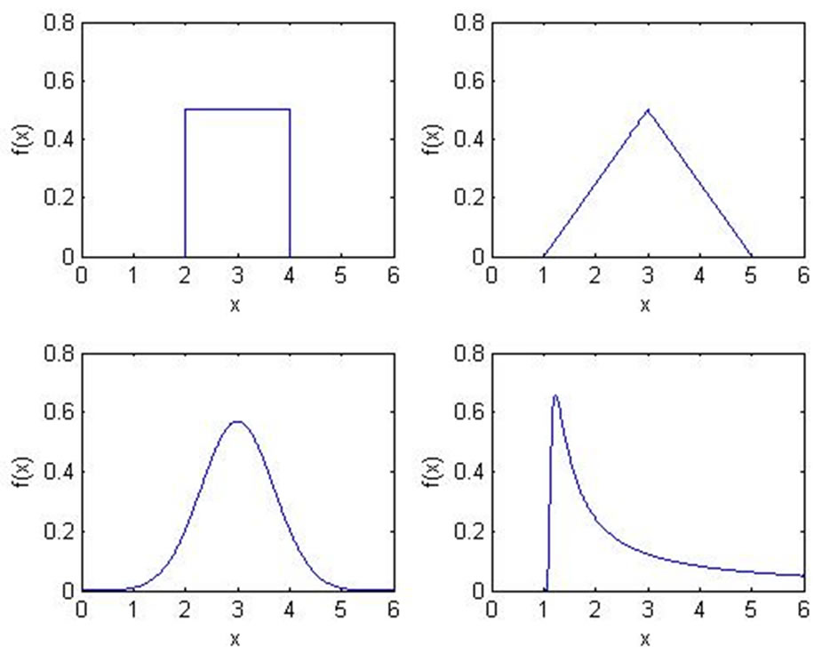
Figure 3. Popular shapes of continuous probability distributions for risk variables: uniform distribution (upper left panel), triangular distribution (upper right panel), normal distribution (lower left panel) and a skewed distribution (lower right panel).
researchers have developed models that incorporate management action into the Monte Carlo simulation, but so far generally lacking sufficient transparency for practitioners and based on a high level of complexity [40].
Another limitation of this generally widely-accepted method is the fact that it also relies on the subjective input of experts with their knowledge and experience. The success of the simulation of the forecast therefore clearly depends on the validity and relevance of the information it is based on. The actions of reviewing estimates, allocating probability weights to values and choosing probability distributions incorporate a high risk of human error.
Despite the overall acceptance of Monte Carlo simulation in the risk analysis literature, some researchers have proposed minor amendments of current Monte Carlo simulation practices in project appraisal.
Balcombe and Smith [15] identified areas where current practices within the Monte Carlo simulation can be improved. Their main objective was to develop a model that was most precise but without being too complex for practical implementation. They propose to include trends, cycles and correlations into the simulation models. For the sake of feasibility, the risk analyst would only have to set “likely bounds” for the variables of interest at the beginning and end of the project duration as well as defining an approximate correlation matrix. This approach possesses the advantage of incorporating additional features like trends, cycles, and correlations, making it a practical and possibly more accurate approach than a normal NPV simulation.
Javid and Seneviratne [93] develop a model to simulate investment risk, using the example of airport parking facility construction and development. This model uses a standard risk management approach by firstly identifying the possible sources of risk on the project. Secondly, probability distributions of certain parameters, which affect the rate of return such as parking demand, are estimated. The model is based on Monte Carlo simulation and aimed to better estimate the impacts of cash flow uncertainties on project feasibility by also including a sensitivity analysis.
Graves [39] discusses different alternatives of probability distributions that can be taken for estimating the project task duration as previously mentioned in Section 2.5. He criticises the commonly used distributions with a finite range as they explicitly exclude the possibility of the task being completed before the minimum duration or beyond the maximum duration limit. In his opinion the basis of a distribution with a finite range is not a realistic assumption for real-world projects, as external and/or internal incidents often have a dynamic stake on the development and process of the project. Due to the dynamics experienced during the course of a project, he gives preference to distributions with an infinite range over bounded distributions (such as the triangular distribution) in Monte Carlo simulations. The main reason for his preference of a duration distribution with infinite range, namely the lognormal distribution, is the possibility of exceeding the project’s maximum duration limit, resulting in a more realistic simulation. Graves [39] also suggests that in creating such a distribution, the project manager should get a base estimate, a contingency amount, and an overrun probability estimate.
Button [94] focuses on improving a more realistic simulation of projects as dealt with in the real-world. His main criticism of the Monte Carlo simulation is that it lacks a multi-project approach, since a single project stands seldom alone in today’s work environment, which is highly complex with projects often being interlinked. Button’s model simulated “both project and non-project work in a multi-project organization” by modelling periodic resource output for all active tasks and for each resource. On the one hand, the advantage of this approach is the enhanced accuracy of this model in multi-project organisations where resources are diluted across many different projects and activities. On the other hand, the disadvantage is its practical implementation due to the model’s complexity and its inexistence in commercially available software packages.
With regard to simulating the NPV of potential investments and projects, Hurley [95] argues that the Monte Carlo simulation’s approach to multi-period uncertainty of the variables is unrealistic for some parameters. He suggests that each parameter should be modelled over time as a Martingale with an additive error term having shrinking variances, eventually making the error variance become smaller in each successive period of the project. He further suggests that this approach results in “more realistic parameter time series that are consistent with the initial assumptions about uncertainty”.
3.4. Real-World State of the Art in the Public Sector
The practical implementation of the described techniques for risk analysis in project appraisal procedures has been thoroughly assessed in the relevant literature. Balcombe and Smith [15] argue that the statistical analysis of the financial revenue estimate before and after completion of a project is either dismissed or subject to a rather general descriptive analysis. Many authors recommend the use of statistical analyses particularly in the light of enhanced and renewed development of micro-computer technologies, providing such approaches more accessible to all project appraisal analysts [12,30,96]. Review of recent studies reveals that a discrepancy between public and private institutions exists when using statistical approaches such as the Monte Carlo Simulation.
Akalu [97] examines how private institutions undertake investment appraisal using a sample of the top 10 British and Dutch companies. The findings indicate that the firms do not apply uniform appraisal techniques throughout the project life cycle and with generally less emphasis on project risk. Seven of the ten assessed companies base their analysis on qualitative methods of measuring project risk. Most companies do not evaluate project risk on continuous matter, but instead apply constant cost of capital across time. This method clearly underestimates the impact risk can expose on projects what may increase the cost of risk in the long term.
Some public institutions such as the World Bank have described their approach to the analysis of risk and uncertainty in their publications, notably Pouliquen [92] and Reutlinger [98]. The World Bank has in addition published several user guidelines and manuals for risk analysis in the project appraisal procedures Belli et al. [99] and Szekeres [100]. Furthermore, the in housedeveloped risk management software “INFRISK” is explained with great detail by Dailami et al. [101]. Created by the Economic Development Institute of the World Bank, INFRISK generates probability distributions for key decision variables (such as the NPV or IRR) in order to analyse a project’s exposure to a variety of market, credit, and performance risks especially for infrastructure finance transactions that involve the private sector. Yet, there is no document that reviews the practical use of INFRISK in general or relative terms.
With regard to scenario analysis, the European Environment Agency (EEA) states that scenario planning faces particular challenges in the public sector. The procedure of long‑term projections is difficult to implement in the compartmentalised environment of modern government and cannot essentially provide a technical adjustment if a project is driven by short-term concerns. The diversity of public organizations’ objectives and interests can also make it difficult to establish one single stakeholder [4] that requires a consensus and common engagement in public sector scenario exercises. Lempert [5] supports the argumentation that scenario analysis methods targeting small groups may not be applicable for large organization with numerous stakeholders. Furthermore, public sector decision-makers face certain constraints such as a diversity of legitimate but competing objectives and social interests.
Applying sensitivity analysis in public sectors also presents the problem that there are no generally accepted rules against which a change in the value of a variable may be tested and to which extend this will impact on the projected result. A major constraint of sensitivity analysis is that it does not take into account how realistic or unrealistic the projected change in the value of a tested variable is [25]. The World Bank prefers a more complex approach to sensitivity analysis by calculating the switching values of all the critical variables rather than just one at a time [102].
3.5. Empirical Results for a Considered Random Sample
Further analysis of literature published by the World Bank indicates that the practical use of quantitative risk analysis has experienced great alterations over the last decades [6,7]. In the 1980s the practical implementation of in-dept quantitative risk analysis methods was even dismissed in favour of sensitivity analysis due to simpler data and computation requirements [8,9]. Reports conducted in the 1990s indicated that although the necessity for quantitative appraisals was still given, its practical use had to be reinstated [10-12]. An evaluation on the present status of quantitative risk analysis implementation could not be found. Nevertheless, a random selection of 20 project appraisal reports from the years 2000 and 2009 shown in Table 2, which were extracted from the World Bank’s vast project appraisal database, reveals that focal project appraisal methods involve simple risk analysis tools like scenario or sensibility analysis. On the other hand, the implementation of deeper and more sophisticated quantitative approaches to the evaluation of processes and financial or economic risk factors still seems to be underrepresented. These results allow the question, if risk analysis (with or without the use of INFRISK) is yet a standard part of the project appraisal procedure. An earlier study was conducted by Pohl and Mihaljek [103] who analysed the World Bank’s experience with project evaluation for a sample of 1015 projects. Their assessments reveal that the World Bank’s appraisal estimates of a project’s revenue are too optimistic and thus advocate for giving the analytical treatment of project risks more attention in practice, although it must be acknowledged that crucial developments— most notably in computer technologies—have occurred since the survey was conducted in 1992. It is therefore possible that the appraisal of some of the 1,015 assessed projects would nowadays include more quantitative risk analysis techniques.
3.6. Recommendations for Risk Analysis in Project Appraisal
The Asian Development Bank is a further example of a public organization that explains the use of risk analysis in their guidelines for practitioners [104]. It recommends that quantitative risk analysis should mainly be carried
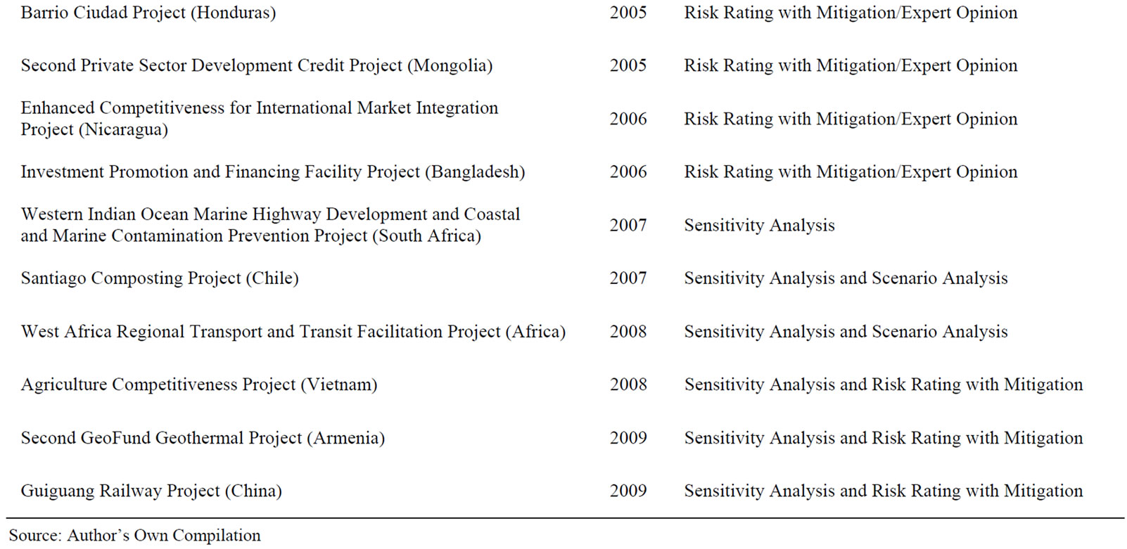
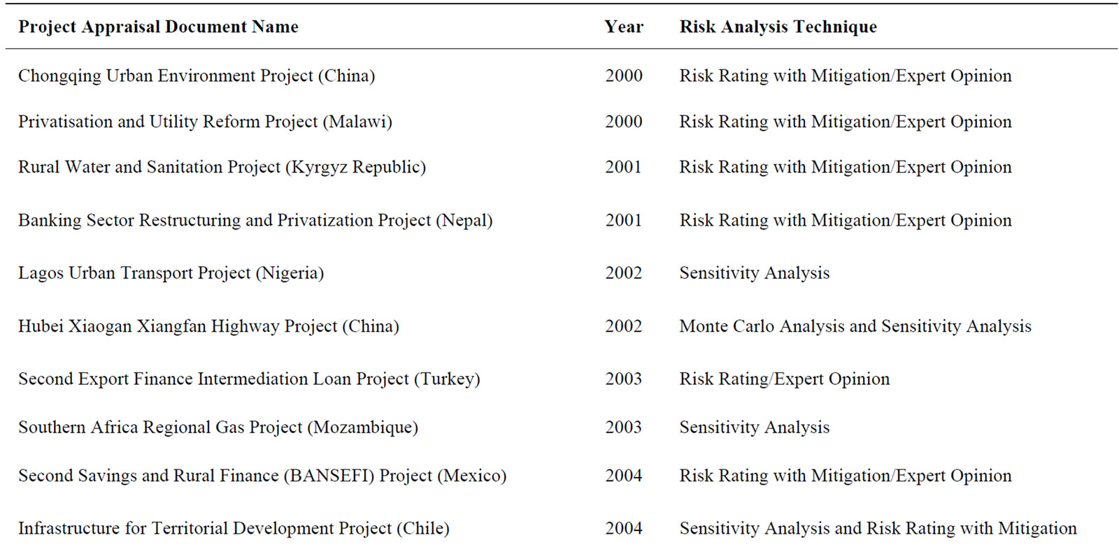
Table 2. Random Sample of projects and applied risk analysis technique from World Bank project appraisal database.
out for large and marginal projects. Furthermore, it states that numerous projects involve risks that cannot be readily quantified such as political or social risks. According to the Asian Development Bank [104], whilst it is complex to insert such risks into risk analysis, these should be considered and included alongside the conclusions of the overall risk analysis.
The World Health Organization advises how information on uncertainty should be communicated to policy makers [105]. The use of probabilistic uncertainty analysis using Monte Carlo simulations is suggested given the generally existing and prevailing scarcity of sampled data on public health interventions costs and effects in high-risk project environments including developing countries.
Notwithstanding limitations to effective statistical analyses within the public sector, Fao and Howard [13] argue that many public organizations (including government departments) have institutionalised scenarioplanning exercises to anticipate the impact of risks and the estimation of future trends of external influences. Nevertheless, the authors point out the potential setbacks of these approaches including methodological rigour, hence recommending the use of the Monte Carlo Simulation.
Despite more feasible application of the Monte Carlo simulation due to modern micro-computer technology, some studies have proposed alternatives to measuring the impact of project risks using this technique. Skitmore and Ng [106] suggest a simplified calculation technique aimed at reducing the methodological complexity of the Monte Carlo Simulation and other analytical approaches. However, their calculation method has been criticised for a lack of validated results as against those derived by the Monte Carlo Simulation and other analytical approaches [14].
Lorterapong and Moselhi [107] favoured the use of fuzzy sets theory in order to quantify the imprecision of expert statements. According to the authors, fuzzy set theory enables the management to represent stochastic or imprecise activity durations, calculate scheduling parameters, and interpret the fuzzy results that are generated through the calculations. They also argued that although the Monte Carlo simulation requires complicated calculations, these have been widely eliminated by advancements in computing power and the availability of Monte Carlo simulation software. It is rather the case that readily available fuzzy sets calculation tools are lacking in the market.
Cho and Yum [108] developed a new analytical approach that estimated the criticality index of a task as a function of the task’s expected duration. They claimed that their approach was more advanced than a Monte Carlo simulation because it was computationally more efficient, requiring less iteration than direct simulation. This approach is more justifiable for extremely large project networks, but has a clear disadvantage in terms of practicality as it lacks readily available tools for project appraisal analysts.
4. Conclusions
In an increasingly dynamic world, commercial, financial, and political organizations are more exposed to external influences, making it difficult to project a stable base for the future of their activities and their organization as a whole. Risk analysis has proven to be a useful tool that has merited increased use in investment appraisal procedures, particularly where uncertainty in key performance and benefit parameter projections requires decisive efforts and decisions.
Risk analysis tools, such as the Monte Carlo Simulation, have the potential to enrich in both quantitative and qualitative terms the information on which project decision-making is ultimately based on. Overall benefits of risk analysis tools encompass their capacity to expand the attributes of a cost-benefit analysis beyond its rather static calculation of key performance and benefit parameters (such as the NPV), taking into consideration the long-term perspective of a sufficient risk-return profile. Risk analysis, in particular the technique of Monte Carlo simulation, can act as a preliminary estimation of the feasibility of an investment opportunity prior to a full and high-cost assessment such as a feasibility study being conducted, thus constraining the costs of prior analysis and assessment in order to avoid significant loss of future income.
Despite the evolution of risk analysis tools over more than six decades, there remains an ongoing debate about specific tool efficiency and application in the real world. Risk analysis methods lack methodological rigour in their practical application; repeatedly their operation is limited within the constraints of human knowledge and computational technology. As computational technology has experienced a steep progress in technical and operational attributes, the major limitations of risk-analysis methods lie within the determining factors of human knowledge and historic data. Other significant limitations are considered to include estimating adequate project duration and the cohesive selection of an accurate probability distribution. A general inability to take into account the influence of factors whose future influence will be significant, but that are presently below the level of detection is a significant limitation of risk analysis. Thus, it is often recommended to rely solely on traditional scenario-planning techniques, as experts would be able to consider and provide estimates of the outcome of such undeterminable factors within the project appraisal period.
A review of the relevant and available literature on risk analysis techniques has revealed that Monte Carlo Simulation presently enjoys the highest recognition in the theoretical assessment of tools for the construction of future scenarios for financial investment projects. The results of the simulation are quantifiable, assisting decision-makers and project managers to make appropriate investment decisions and to avoid unrealistic project expectations. Nonetheless, it is essential to mention that, in addition to the above-mentioned drawbacks, Monte Carlo Simulation is presently still experiencing only limited practical appliance in the real world. Despite its attributes and continuous improvements in computational simulation software, it is still not considered a popular tool within current project management practice in both private and public organizations. In particular for the public sector, practical implementation of Monte Carlo simulation in the appraisal procedure of investment projects has not fully occurred to date. This is mostly due to the technique’s statistical nature and a general lack of capacity to adequately or appropriately conduct these. A literature review and preliminary assessment of published project documents reveal that public organizations still prefer to use simple tools such as cost-benefit analysis, alongside sensitivity and scenario analysis in estimating future outcomes of public investment projects.
This situation is certainly unfortunate considering the often large investment sums and the substantial external effect public projects can have not only on the area of investment but also on the financial and economic performance of the donor organization. With the vast number of diverse stakeholders involved in such investment projects and their potentially competing objectives and social interests, the application of traditional scenario analysis tools and the Delphi technique may be rather cumbersome and long-winded. The use of Monte Carlo simulation and other quantitative approaches like e.g. the mentioned fuzzy analysis should be considered as helpful tools for revealing and evaluating potential risks. A reason for the so far rather limited use of these techniques in practical applications may also be the essentially political processes generally associated with public investment decisions. However, given the often substantive amount of tax money that is used for the financing public investment, it would stand to reason to minimise the possibility of misdirected investments by an appropriate examination of potential outcomes. This is true even though public organizations are not following an entire profit-oriented mission. Based on the conducted review of the literature, it is evident that deeper and more sophisticated quantitative approaches to the evaluation of processes and financial or economic risk factors should be beneficial. This also suggests a higher number of practical implementations of these techniques for project appraisal of public sector institutions.
5. References
[1] M. Florio, U. Finzi, M. Genco, F. Levarlet, S. Maffii, A. Tracogna and S. Vignetti, “Guide to Cost-Benefit Analysis of Investment Projects: Structural Funds-ERDF, Cohesion Fund and ISPA,” 3rd Edition, DG Regional Policy, European Commission, Brussels, 2002.
[2] W. J. H. van Groenendaal and J. P. C. Kleijnen, “On the Assessment of Economic Risk: Factorial Design Versus Monte Carlo Methods,” Journal of Reliability Engineering and Systems Safety, Vol. 57, No. 1, 1997, pp. 91-102. doi:10.1016/S0951-8320(97)00019-7
[3] Environmental Assessment Institute, “Risk and Uncertainty in Cost Benefit Analysis,” Toolbox Paper, Institut for Miljøvurdering, Copenhagen, 2006.
[4] E. A. Parson, V. R. Burkett, K. Fisher-Vanden, D. Keith, L. O. Mearns, H. M. Pitcher, C. E. Rosenzweig and M. D. Webster, “Global-Change Scenarios: Their Development and Use,” Sub-Report, United States Climate Change Science Program and the Subcommittee on Global Change Research, 2007.
[5] R. Lempert, “Can Scenarios Help Policymakers Be Both Bold and Careful?” In: F. Fukuyama, Ed., Blindside: How to Anticipate Forcing Events and Wild Cards in Global Politics, Brookings Institution Press, Washington DC, 2007.
[6] I. M. D. Little and J. A. Mirrlees, “Risk Uncertainty and Profit,” Project Appraisal and Planning for Developing Countries, Heinemann, London, 1994.
[7] S. Devarajan, L. Squire and S. Suthirwart-Narueput, “Reviving Project Appraisal at the World Bank, Policy Research Working Paper No. 1496,” Public Economics Division, Policy Research Department, World Bank, Washington DC, 1995.
[8] J. P. Gittinger, “Economic Analysis of Agricultural Projects,” 2nd Edition, The Johns Hopkins University Press, Baltimore, Maryland, 1982.
[9] Overseas Development Administration, “A Guide to Road Project Appraisal,” Overseas Road Note No. 5, London, 1988.
[10] D. G. Davies, (ed.), “The Economic Evaluation of Projects,” Papers from a Curriculum Development Workshop, World Bank, Washington DC, 1996.
[11] C. Kirkpatrick, “The Rise and Fall of Cost Benefit Analysis: The Role of Project Appraisal in Managing Development Projects,” In: F. Analoui, Ed., The Realities of Managing Development Projects, Avebury, Aldershot, 1994.
[12] J. Weiss, “Project Failure: The Implications of a 25 Percent Rule,” In: C. Kirkpatrick and J. Weiss, Cost-Benefit Analysis and Project Appraisal in Developing Countries, Edward Elgar, Cheltenham, 1996.
[13] R. Fao and M. Howard, “Use of Monte Carlo Simulation for the Public Sector: An Evidence-Based Approach to Scenario Planning, the Market Research Society,” International Journal of Market Research, Vol. 48, No. 1, 2006, pp. 27-48.
[14] Y. H. Kwak and L. Ingall, “Exploring Monte Carlo Simulation Applications for Project Management,” Risk Management, Vol. 9, 2007, pp. 44-57. doi:10.1057/palgrave.rm.8250017
[15] K. Balcombe and L. Smith, “Refining the Use of Monte Carlo Techniques for Risk Analysis in Project Planning,” Journal of Development Studies, Vol. 36, No. 2, 1999, pp. 113-135. doi:10.1080/00220389908422623
[16] F. H. Knight, “Risk, Uncertainty and Profit,” Houston Mifflin, Boston, 1921.
[17] J. F. Weston, “The Profit Concept and Theory: A Restatement,” The Journal of Political Economy, Vol. 62, No. 6, 1954, pp. 152-170. doi:10.1086/257499
[18] G. Stigler, “Frank Knight,” In: J. Eatwell, M. Milgate and P. Newman, Eds., The New Palgrave Dictionary of Economics, Stockton Press, New York, 1987.
[19] M. Friedman, “Price Theory: A Provisional Text,” Aldine, Chicago, 1976.
[20] S. F. le Roy and D. Singell, “Knight on Risk and Uncertainty,” The Journal of Political Economy, Vol. 95, No. 2, 1987, pp. 394-406. doi:10.1086/261461
[21] A. Jaafari, “Management of Risks, Uncertainties and Opportunities on Projects: Time for a Fundamental Shift,” International Journal of Project Management, Vol. 19, No. 2, 2001, pp. 89-101. doi:10.1016/S0263-7863(99)00047-2
[22] N. Piyatrapoomi, A. Kumar and S. Setunge, “Framework for Investment Decision-Making under Risk and Uncertainty for Infrastructure Asset Management,” Research in Transportation Economics, Vol. 8, No. 1, 2004, pp. 199- 214. doi:10.1016/S0739-8859(04)08010-2
[23] D. Vose, “Risk Analysis—A Quantitative Guide,” 2nd Edition, John Wiley & Sons Ltd., Chichester, 2000.
[24] H. van Greuning and S. Brajovic-Bratanovic, “Banking Risk Analysis and Management,” Irecson Publishing House, Bucharest, 2003. doi:10.1596/0-8213-5418-3
[25] S. Savvides, “Risk Analysis in Investment Appraisal,” Project Appraisal, Vol. 9, No. 1, 1994, pp. 1-30.
[26] C. B. Chapman and S. C. Ward, “Project Risk Management: Processes, Techniques and Insights,” 2nd Edition, John Wiley & Sons, Chichester, 2003.
[27] D. B. Hertz and H. Thomas, “Risk Analysis and Its Applications,” John Wiley, Chichester, 1983.
[28] I. Dikmen, M. T. Birgonul, C. Anac, J. H. M. Tah and G. Aouad, “Learning from Risks: A Tool for Post-Project Risk Assessment,” Automation in Construction, Vol. 18, No. 1, 2008, pp. 42-50. doi:10.1016/j.autcon.2008.04.008
[29] D. Vose, “Risk Analysis—A Quantitative Guide,” 3rd Edition, John Wiley & Sons Ltd., Chichester, 2008.
[30] M. Florio, “Cost-Benefit Analysis and the Rates of Return of Development Projects: An International Comparison,” Centro Studi Luca d’Agliano Development Studies Working Papers No. 182, 2003.
[31] B. Jafarizadeh and R. Khorshid-Doust, “A Method of Project Selection Based on Capital Asset Pricing Theories in a Framework of Mean-Semideviation Behaviour,” International Journal of Project Management, Vol. 26, No. 6, 2007, pp. 612-619.
[32] A. Saltelli, et al., “Global Sensitivity Analysis: The Primer,” John Wiley & Sons Ltd., Chichester, 2004.
[33] A. E. Boardman, D. H. Greenberg, A. R. Vining and D. L. Weimer, “Cost Benefit Analysis: Concepts and Practice,” 3rd Edition, Prentice Hall, Upper Saddle River, 2006.
[34] T. Merna and D. V. Storch, “Risk Management of Agricultural Investment in a Developing Country Utilising the CASPAR Program,” International Journal of Project Management, Vol. 18, No. 5, 2000, pp. 349-360. doi:10.1016/S0263-7863(99)00050-2
[35] A. H. Russell, “Cash Flows in Networks,” Management Science, Vol. 16, No. 5, 1970, pp. 357-373. doi:10.1287/mnsc.16.5.357
[36] R. C. Grinold, “The Payment Scheduling Problem,” Naval Research Logistics Quarterly, Vol. 19, No. 1, 1972, pp. 123-136. doi:10.1002/nav.3800190110
[37] S. E. Elmaghraby and W. S. Herroelen, “The Scheduling of Activities to Maximize the Net Present Value of Projects,” European Journal of Operational Research, Vol. 49, 1990, pp. 35-49. doi:10.1016/0377-2217(90)90118-U
[38] R. Etgar, A. Shtub and L. J. Leblanc, “Scheduling Projects to Maximise Net Present Value—The Case of Time-Dependent, Contingent Cash Flows,” European Journal of Operational Research, Vol. 96, No. 1, 1995, pp. 90-96. doi:10.1016/0377-2217(95)00382-7
[39] R. Graves, “Open and Closed: The Monte Carlo Model,” PM Network, Vol. 15, No. 12, 2001, pp. 37-41.
[40] T. Williams, “The Contribution of Mathematical Modelling to the Practice of Project Management,” IMA Journal of Management Mathematics, Vol. 14, No. 1, 2003, pp. 3-30. doi:10.1093/imaman/14.1.3
[41] W. C. Baum and S. M. Tolbert, “Investing in Development. Lessons of World Bank Experience,” Oxford University Press, Oxford, 1985.
[42] G. Koop, D. Poirier and J. Tobias, “Bayesian Econometric Models,” Cambridge University Press, Cambridge, 2007.
[43] T. Bedford and R. Cooke, “Probabilistic Risk Analysis: Foundations and Methods,” Cambridge University Press, Cambridge, 2001.
[44] R. A. Brealey and S. C. Myers, “Principles of Corporate Finance,” 6th Edition, Irwin McGraw-Hill, Boston, 2000.
[45] L. Trigeorgis, “Real Options: Managerial Flexibility and Strategy in Resource Allocation,” MIT Press, Cambridge, 1997.
[46] P. N. Smith, S. Sorensen and W. R. Wickens, “Macroeconomic Sources of Equity Risk,” Discussion Papers 03/13, Department of Economics, University of York, York, 2003.
[47] N. M. L. Barnes, “How to Allocate Risks in Construction Contracts,” International Journal of Project Management, Vol. 1, No. 1, 1983, pp. 24-28. doi:10.1016/0263-7863(83)90034-0
[48] S. G. Kahn, “Partners in Risk,” Cost Incentive Development Contracts, ESA Bulletin, Vol. 26, 1981, pp. 48-53.
[49] J. Lintner, “Valuation of Risky Assets and the Selection of Risky Investments in Stock Portfolios and Capital Budgets,” Review of Economics and Statistics, Vol. 47, No. 1, 1965, pp. 13-37.
[50] W. F. Sharpe, “Capital Asset Prices: A Theory of Market Equilibrium under Conditions of Risk,” Journal of Finance, Vol. 19, No. 3, 1964, pp. 425-442. doi:10.2307/2977928
[51] A. Huchzermeier and C. H. Loch, “Project Management under Risk: Using the Real Options Approach to Evaluate Flexibility in R & D,” Management Science, Vol. 47, No. 1, 2001, pp. 85-101. doi:10.1287/mnsc.47.1.85.10661
[52] W. E. Walker, “Policy Analysis: A Systematic Approach to Supporting Policymaking in the Public Sector,” Journal of Multi-Criteria Decision Analysis, Vol. 9, No. 1-3, 2000, pp. 11-27. doi:10.1002/1099-1360(200001/05)9:1/3<11::AID-MCDA264>3.0.CO;2-3
[53] P. W. F. van Notten, J. Rotmans, M. B. A. van Asselt and D. A. Rothman, “An Updated Scenario Typology,” Futures, Vol. 35, No. 5, 2003, pp. 423-443. doi:10.1016/S0016-3287(02)00090-3
[54] R. Bradfield, G. Wright, G. Burt, G. Cairns and K. van der Heijden, “The Origins and Evolution of Scenario Techniques in Long Range Business Planning,” Futures, Vol. 37, 2006, pp. 795-812. doi:10.1016/j.futures.2005.01.003
[55] P. Schwartz, “The Art of the Long View,” Doubleday/Currency, New York, 1991.
[56] K. van der Heijden, “Scenarios: The Art of Strategic Conversation,” John Wiley and Sons, Chichester, 1996.
[57] L. Börjeson, M. Höjer, K. Dreborg, T. Ekvall and G. Finnveden, “Scenario Types and Techniques: Towards a User’s Guide,” Futures, Vol. 38, No. 7, 2006, pp. 723- 739.
[58] P. Bishop, A. Hines and T. Collins, “The Current State of Scenario Development: An Overview of Techniques,” Foresight, Vol. 9, No. 1, 2007, pp. 5-25. doi:10.1108/14636680710727516
[59] European Environment Agency, “Looking Back on Looking Forward: A Review of Evaluative Scenario Literature,” EEA Technical Report, No. 3, 2009.
[60] G. Wright, M. J. Lawrence and F. Collopy, “The Role and Validity of Judgment in Forecasting,” International Journal of Forecasting, Vol. 12, No. 1, 1996, pp. 1-8. doi:10.1016/0169-2070(96)00674-7
[61] G. Rowe and g. Wright, “The Delphi Technique as a Forecasting Tool: Issues and Analysis,” International Journal of Forecasting, Vol. 15, No. 3, 1999, pp. 53-375.
[62] H. A. Linstone and M. Turoff, “The Delphi Method: Techniques and Applications,” Addison-Wesley, London, 1975.
[63] A. Lock, “Integrating Group Judgments in Subjective Forecasts,” In: G. Wright and P. Ayton, Eds., Judgmental Forecasting, Wiley, Chichester, 1987.
[64] F. J. Parenté and J. K. Anderson-Parenté, “Delphi Inquiry Systems,” In: G. Wright and P. Ayton, Eds., Judgmental Forecasting, Wiley, Chichester, 1987.
[65] T. R. Stewart, “The Delphi Technique and Judgmental Forecasting,” Climatic Change, Vol. 11, 1987, pp. 97-113. doi:10.1007/BF00138797
[66] G. Rowe, G. Wright and F. Bolger, “The Delphi Technique: A Re-Evaluation of Research and Theory,” Technological Forecasting and Social Change, Vol. 39, No. 3, 1991, pp. 235-251. doi:10.1016/0040-1625(91)90039-I
[67] N. C. Dalkey and O. Helmer, “An Experimental Application of the Delphi Method to the Use of Experts,” Management Science, Vol. 9, No. 3, 1963, pp. 458-467. doi:10.1287/mnsc.9.3.458
[68] W. C. Wedley, “New Uses of Delphi in Strategy Formulation,” Long Range Planning, Vol. 10, No. 6, 1977, p. 70. doi:10.1016/0024-6301(77)90011-5
[69] F. J. Parenté, J. K. Anderson, P. Myers and T. O’Brien, “An Examination of Factors Contributing to Delphi Accuracy,” Journal of Forecasting, Vol. 3, No. 2, 1984, pp. 173-182. doi:10.1002/for.3980030205
[70] G. Rowe and G. Wright, “The Impact of Task Characteristics on the Performance of Structured Group Forecasting Techniques,” International Journal of Forecasting, Vol. 12, No. 1, 1996, pp. 73-89. doi:10.1016/0169-2070(95)00658-3
[71] L. L. Leape, M. A. Freshour, D. Yntema and W. Hsiao, “Small Group Judgment Methods for Determining Resource Based Relative Values,” Medical Care, Vol. 30, No. 11, 1992, pp. NS28-NS39. doi:10.1097/00005650-199211001-00003
[72] F. C. Miner, “A Comparative Analysis of Three Diverse Group Decision Making Approaches,” Academy of Management Journal, Vol. 22, No. 1, 1979, pp. 81-93. doi:10.2307/255480
[73] C. S. Huang, Y. Lin and C. Lin, “Determination of Insurance Policy Using a Hybrid Model of AHP, Fuzzy Logic, and Delphi Technique: A Case Study,” WSEAS Transactions on Computers, Vol. 7, No. 6, 2008, pp. 660-669.
[74] H. Sackman, “Delphi Critique,” Lexington Books, Lexington, 1975.
[75] M. J. Bardecki, “Participants’ Response to the Delphi Method: An Attitudinal Perspective,” Technological Forecasting and Social Change, Vol. 25, 1984, pp. 281- 292. doi:10.1016/0040-1625(84)90006-4
[76] J. O. Berger, “Statistical Decision Theory and Bayesian Analysis,” Springer, New York, 1985.
[77] H. Bühlmann and A. Gisler, “A Course in Credibility Theory and Its Applications,” Springer, Berlin, 2005.
[78] S. T. Rachev, J. Hsu, B. Bagasheva and F. Fabozzi, “Bayesian Methods in Finance,” Wiley, New York, 2008.
[79] P. V. Shevchenko and M. V. Wüthrich, “The Structural Modelling of Operational Risk via Bayesian Inference: Combining Loss Data with Expert Opinions,” Journal of Operational Risk, Vol. 1, No. 3, 2006, pp. 3-26.
[80] S. Trück and C. Truong, “Catastrophic Risks and Optimal Climate Change Adaptation Strategies at the Local Level,” Working Paper, Macquarie University, Sydney, Australia, 2009.
[81] B. Clemson, Y. Tang, J. Pyne and R. Unal, “Efficient Methods for Sensitivity Analysis,” System Dynamics Review, Vol. 11, No. 1, 1995, pp. 31-49. doi:10.1002/sdr.4260110104
[82] T. G. Eschenbach and R. J. Gimpel, “Stochastic Sensitivity Analysis,” The Engineering Economist, Vol. 35, No. 4, 1990, pp. 305-321. doi:10.1080/00137919008903024
[83] D. M. Hamby, “A Review of Techniques for Parameter Sensitivity Analysis of Environmental Models,” Environmental Monitoring and Assessment, Vol. 32, No. 2, 1994, pp. 135-154. doi:10.1007/BF00547132
[84] K. J. Lomas and H. Eppel, “Sensitivity Analysis Techniques for Building Thermal Simulation Programs,” Energy and Buildings, Vol. 19, 1992, pp. 21-44. doi:10.1016/0378-7788(92)90033-D
[85] S. G. Tzafestas, N. Theodorou and A. Kanellakis, “Recent Advances in the Stability Analysis of Multidimensional Systems,” Information and Decision Technologies, Vol. 14, 1988, pp. 195-211
[86] D. J. Pannell, “Sensitivity Analysis of Normative Economic Models: Theoretical Framework and Practical Strategies,” Agricultural Economics, Vol. 16, No. 2, 1997, pp. 139-152. doi:10.1016/S0169-5150(96)01217-0
[87] F. Canova, “Sensitivity Analysis and Model Evaluation in Simulated Dynamic General Equilibrium Economies,” International Economic Review, Vol. 36, No. 2, 1995, pp. 477-501. doi:10.2307/2527207
[88] G. W. Harrison and H. D. Vinod, “The Sensitivity Analysis of Applied General Equilibrium Models: Completely Randomised Factorial Sampling Designs,” The Review of Economics and Statistics, Vol. 74, No. 2, 1992, pp. 357-362. doi:10.2307/2109672
[89] P. Javanovic, “Application of Sensitivity Analysis in Investment Project Evaluation under Uncertainty and Risk,” International Journal of Project Management, Vol. 17, No. 4, 1999, pp. 217-222. doi:10.1016/S0263-7863(98)00035-0
[90] G. E. P. Box, W. G. Hunter and J. S. Hunter, “Statistics for Experimenters: An Introduction to Design, Data Analysis, and Model Building,” John Wiley & Sons, New York, 1978.
[91] Z. M. Christopher, “Monte Carlo Simulation, Quantitative Applications in the Social Sciences,” Sage University Papers Series, No. 116, 1997.
[92] L. Y. Pouliquen, “Risk Analysis in Project Appraisal,” Staff Occasional Paper, The World Bank, Washington DC, 1970.
[93] M. Javid and P. Seneviratne, “Investment Risk Analysis in Airport Parking Facility Development,” Journal of Construction Engineering and Management, Vol. 126, No. 4, 2000, pp. 298-305. doi:10.1061/(ASCE)0733-9364(2000)126:4(298)
[94] S. Button, “Project Duration Prediction Using a Monte Carlo Simulation of the Periodic Output of the Project Resources,” Monte Carlo Methods and Applications, Vol. 9, No. 3, 2003, pp. 217-225. doi:10.1515/156939603322728987
[95] W. Hurley, “On the Use of Martingales in Monte Carlo Approaches to Multiperiod Parameter Uncertainty in Capital Investment Risk Analysis,” The Engineering Economist, Vol. 43, No. 2, 1998. doi:10.1080/00137919808903195
[96] R. Clarke and A. Low, “Risk Analysis in Project Planning: A Simple Spreadsheet Application Using MonteCarlo Techniques’,” Project Appraisal, Vol. 8, No. 3, 1993.
[97] M. M. Akalu, “The Process of Investment Appraisal: The Experience of 10 Large British and Dutch Companies,” International Journal of Project Management, Vol. 21, No. 5, 2002, pp. 355-362. doi:10.1016/S0263-7863(02)00051-0
[98] S. Reutlinger, “Techniques for Project Appraisal under Uncertainty,” World Bank Staff Occasional Papers No. 10, Johns Hopkins Press, Baltimore, 1970.
[99] p. belli, J. R. Anderson, j. a. Dixon and j. p. tan, “Economic Analysis of Investment Operations: Analytical Tools and Practical Applications,” World Bank Institute Development Studies, Washington DC, 2001.
[100] S. Szekeres, “Considering Uncertainty in Project Appraisal,” EDI, World Bank, Washington DC, 1986.
[101] M. Dailami, I. Lipkovich and J. van Dyk, “INFRISK, a Computer Simulation Approach to Risk Management in Infrastructure Project Finance Transactions,” World Bank Policy Research Working Paper, the World Bank Economic Development Institute, Washington DC, 1999.
[102] World Bank, “Risk & Uncertainty Analysis, Transport Economics,” Transport Note No. TRN-7, Policy and Poverty Thematic Group, 2005.
[103] G. Pohl and D. Mihaljek, “Project Evaluation and Uncertainty in Practice: A Statistical Analysis of Rate-of-Return Divergences of 1015 World Bank Projects,” World Bank Economic Review, Vol. 6, No. 2, 1992, pp. 255-277. doi:10.1093/wber/6.2.255
[104] Asian Development Bank, “Guidelines for the Economic Analysis of Guidelines for the Economic Analysis of Projects,” Economics and Development Resource Centre, On-Line Publication from ADB Homepage Site, 1999.
[105] R. Baltussen, R. Hultubessy, D. Evans and C. Murray, “Uncertainty in Cost-Effectiveness Analyses: Probabilistic Uncertainty Analysis and Stochastic League Tables,” International Journal of Technology Assessment in Health Care, Vol. 18, No. 1, 2002, pp. 112-119.
[106] M. Skitmore and S. Ng, “Analytical and Approximate Variance of Total Project Cost,” Journal of Construction Engineering and Management, Vol. 128, No. 5, 2002, pp. 456-460. doi:10.1061/(ASCE)0733-9364(2002)128:5(456)
[107] P. Lorterapong and O. Moselhi, “Project-Network Analysis Using Fuzzy Sets Theory,” Journal of Construction Engineering and Management, Vol. 122, No. 4, 1996, pp. 308-318. doi:10.1061/(ASCE)0733-9364(1996)122:4(308)
[108] J.-G. Cho and B.-J. Yum, “Functional Estimation of Activity Criticality Indices and Sensitivity Analysis of Expected Project Completion Time,” Journal of the Operational Research Society, Vol. 55, No. 8, 2004, pp. 850-859. doi:10.1057/palgrave.jors.260173