Journal of Electromagnetic Analysis and Applications
Vol.09 No.11(2017), Article ID:80794,20 pages
10.4236/jemaa.2017.911016
Simulated Experiments for Teaching Mutually-Coupled Circuits CAD Techniques Using Analytic and Finite Element Solutions
Antônio Flavio Licarião Nogueira, Vítor Hörbe Pereira da Costa, Rodolfo Lauro Weinert
Santa Catarina State University, Joinville, Brazil

Copyright © 2017 by authors and Scientific Research Publishing Inc.
This work is licensed under the Creative Commons Attribution International License (CC BY 4.0).
http://creativecommons.org/licenses/by/4.0/


Received: October 7, 2017; Accepted: November 27, 2017; Published: November 30, 2017
ABSTRACT
The paper describes an approach to teaching mutually-coupled circuits CAD techniques to undergraduate students pursuing a degree course in electrical engineering or physics, and explains how a series of simulated experiments may be incorporated into the existing subjects. The simulated experiments make use of a two-dimensional open-access software based on the finite-element method. At the laboratory meetings, the students learn how to set up field problems for solution, and how to examine the results. Simulation tasks based on three axisymmetric open-boundary problems are used to introduce different numeric techniques to compute inductance and magnetic forces. The paper takes the reader to a step-by-step simulation journey, and provides all the basic elements required for further exploration of axially-symmetric systems.
Keywords:
Electromagnetic Engineering Education, Finite Element Method, Inductance, Magnetic Forces, Simulation Software

1. Introduction
In the past, development, analysis and design of electric equipment have used extremely simple analytic methods, supplemented by experience and intuition. As a result, any change in the device’s specifications would be time consuming and difficult to be accommodated by the traditional methods of analysis. The decade of 1980 witnessed an increasing number of electric equipment manufacturers relying on electromagnetic computer-aided design (CAD) packages in their analysis tasks [1] . Also, academic groups have developed their own CAD packages and worked together with manufacturing organizations to jointly perform a broad variety of experimental and simulated work. That new era in computer-aided design has witnessed numerous courses on simulation of electromagnetic fields given to industrial researchers as well as several successful didactical experiences based on the creation of laboratories of simulations.
The literature documents extensive research into the development of computer-assisted educational material to teach physics and engineering. Fortunately, there are excellent surveys intended to aid faculty members in their choices related to curriculum changes and incorporation of innovative educational methods [2] [3] . There are many papers describing new approaches to teach electromagnetics and, almost without exception, these papers advocate the integration of field computation into electromagnetics teaching. The underlying idea is to develop new practical alternatives to the traditional teaching approach to circumvent the difficulties in teaching electromagnetics, regarded as an abstract and difficult subject [4] . Of major note is the work of Lowther and Freeman [5] . The work describes how laboratory courses on field simulation have been devised and implemented in three different universities, and discusses the advantages and disadvantages of finite-element CAD tools in the teaching environment.
Innovations in educational methods and changes in curriculum are usually guided by questions like: (i) to incorporate these developments into the curriculum, should a separate subject be created, or a change in the number of laboratory hours would speed up the process; (ii) which are the relevant considerations for the choice of the instructional software; (iii) which numerical method will more likely be used by the students upon graduation, as research students or practicing professionals.
With these uncertainties in mind, we decided to incorporate a series of simulated experiments into the existing laboratories of subjects around electromagnetics, like basic electromagnetism and electromechanical conversion of energy. The experiments focus on electromagnetic phenomena that are overwhelmingly better explained using field computation, such as: magnetic saturation, magnetic forces and inductance. All experiments are carried out using a two-dimensional open-access simulation software based on the finite-element method [6] . The choice of this numerical method has considered its worldwide popularity as teaching tool as well as its enhanced capability in the analysis of problems involving non-linearity and time-dependent phenomena [7] [8] [9] . An additional argument in favor of this choice is that the finite-element method can now be presented in simple terms, avoiding the rigorous mathematical derivations of variational calculus, and making the method more attractive to students [10] .
The paper describes a set of simulated experiments devised and developed to teach numerical techniques for the calculation of inductance. The experiments place emphasis on demonstrating how to set up field problems for solution, and how to examine the results using selected graphical presentations as well as computation of global quantities like inductance, stored energy and magnetic forces. There are seven experiments all together, wherein three axisymmetric open-boundary physical problems are analyzed in detail.
2. Coaxial Coils Immersed in Air
The first problem consists of calculating values of self-inductance L, mutual inductance M and leakage inductance l of the idealized two coaxial coils’ system shown in Figure 1. This physical system represents one of the simplest closed circuit current distributions, and has long been used to present the relationship between the magnetic flux and the inductance terms associated to coaxial coils in free space. The system consists of two thin circular coils, and both coils have exactly one turn. The lower coil has a radius R = 10.0 cm, and the upper coil has a radius r = 5.0 cm. The axial distance between the center of the two coils is z = 1.0 cm. The solid copper wire used in both coils has a radius rm = 0.0512 cm, the same radius of an 18 AWG conductor, and its electric conductivity is 58 MS/m. For this problem, there is a simple analytical expression for the mutual inductance, expressed in terms of the axial distance, z, between the centers of the two coils,
(1)
where µ0 = 4π ´ 10−7 H/m is the magnetic permeability of free space [11] . This expression is used to check the accuracy of different calculation methods. The formula expressed in (1) is approximate, and its accuracy depends on the geometric dimensions of the coils. The numeric estimates for the self-inductance, L, of individual coils are compared to the analytical formula originally presented by Kirchhoff [11] ,
(2)

Figure 1. Two coaxial coils with different radii and same wire cross section.
The variation of the mutual inductance with respect to the axial distance z may be used to derive the analytic expression for the axially-directed magnetic force, F, between the two coils carrying currents I1 and I2,
(3)
with the minus sign indicating attraction. The complete derivation of formulae expressed in (1) and (3) appears in Appendix A.
Open-Boundary Problems
The calculation of inductance terms of coaxial coils immersed in air is an open boundary problem. To obtain a solution using the finite element technique, it is necessary to convert the open boundary problem into a closed one by main force. This can be done by creating an artificial boundary sufficiently distant of the device under analysis. The simplest open-boundary technique is truncation of outer boundaries, a technique based on the assumption that, at the artificial boundary, the vector potential A or its normal derivative ¶A/¶n will be close to zero. To minimize the numerical error due to “truncation” in the computation of the potentials, it is necessary to place the exterior boundary sufficiently far away from the device [12] .
The problem of the coaxial coils may then be artificially closed by an exterior spherical boundary. In axisymmetric problems, a spherical boundary is generated by rotating a semicircular region about the axis of symmetry. According to the general rule of thumb for locating the outer boundary, the radius of this external semicircular boundary should be at least 50 cm, i.e., approximately five times the distance between the most remote coil and the center of the geometry [13] . In the numerical model described in the following, the analysis domain is bound by a semicircular region with 100 cm of radius. This large area of empty space surrounding the coils will allow extra flexibility for the definition of similar problems with increasing radii in the same analysis domain, and leaving the coils’ region practically unaffected by truncation error.
3. Finite-Element Model
3.1. Problem Definition
The definition of a finite-element problem always involves a large amount of input data, and the user must select the key features of the analysis task. Initially, it is necessary to select the type of solver and, implicitly define the primary quantity of calculation, i.e., magnetic vector potential A for magnetics problems, and electric potential V for electrostatic and current-flow problems. This is followed by the choice of the length unit, frequency of excitation and kind of symmetry to be exploited, either planar or rotational. For present considerations of inductance calculations, we shall restrict our attention to magnetostatic problems with rotational symmetry. The excitations are defined in terms of electric currents, and the frequency of operation is zero.
3.2. Problem Geometry
The definition of the problem geometry may start by inserting the end-points that define the two corners of the solution geometry shown in Figure 2(a). For a solution domain centered at (r, z) = (0, 0), the corners are located at (r, z) = (0, −100) and (r, z) = (0, 100) with length units in centimeter. This pair of end-points must be connected using a line-segment, followed by an arc of 180° and 100 cm of radius to create the external boundary G. As part of the mesh artifact, an additional arc of 180˚ and 60 cm of radius centered at (r, z) = (0, 0) is included in the geometry. This arc works as an artificial “air-air” boundary, and has been included to avoid a very large number of triangles in the mesh. To complete the problem geometry, it is still necessary to draw two regions representing the cross-section of the wire used in each coil.
3.3. Problem Assembly
The definition of the problem geometry is followed by a series of tasks known as problem assembly. These tasks state the correlation between region labels and materials, and allow the specification of boundary values and sources of energy. The problem assembly involves four types of data specification: material property, boundary property, point property and circuit property.
3.4. Materials and Boundary Conditions
This numeric model contains four regions representing two coils and two layers of air, and a label must be placed in each region. Next, it is necessary to associate material properties with region labels, “air” for the two layers of air, “copper” for

Figure 2. (a) Geometrical dimensions in cm; (b) maximum triangles’ edge size in each region with values in cm.
the two circles representing the coils. A boundary property with prescribed potential A = 0 must be created and assigned to the external semicircle that bounds the analysis domain. Along the axis of symmetry, the condition A = 0 is automatically enforced in magnetics axisymmetric problems.
3.5. Coil Currents
For each coil, it is necessary to create a “circuit property” that specifies the coil current in units of ampere, its direction and number of turns. It is important to observe that, a circuit property must be assigned to all coils, even for the coils that carry no current. By using circuit properties, the value of flux linkage with each individual coil will become automatically available at the post processing operations. The value of the flux linkage with the unexcited coil is an essential information for the calculation of mutual inductance by the method of flux linkage, as discussed later in the first experiment.
3.6. Mesh Refinement
The method employed to control the level of discretization in each region is based on the specification of a parameter, δ, known as “edge size”. This parameter defines a constraint on the largest possible size of the elements’ edges allowed in that region. The mesh generator Triangle [14] attempts to fill each selected region with nearly equilateral triangles. According to the illustration of Figure 2(b), the two regions representing the conductors are discretized with edge size δ = 0.01 cm, the first layer of air with edge size δ = 0.1 cm, and the second layer of air with edge size δ = 1.0 cm. This level of discretization leads to a mesh with 595697 nodes and 1189909 triangular elements.
4. Experiments
Although a considerable effort is necessary in establishing a numeric model, variations of the problem configuration may be readily tested without having to restart the entire job. So, information present in the laboratory guides should state clearly which features of mesh construction, as well as specification of boundary conditions and sources of energy will lead to extra flexibility for altering material properties and defining sequences of similar problems [15] . A great deal of effort can be saved if we work with one numeric model and a series of problems defined on that model. With this in mind, we have decided to base our laboratory classes on simple physical devices, and leave the variations of the problem with increasing degree of complexity for the homework, carried out as a peer-mentoring activity. Assessment to the students’ performance is based on written reports. The set of graded exercises proposed in the following is indicative of the type of problems students will meet in their work.
4.1. Inductance Calculations via Flux Linkage Approach
Compute the inductance terms of the two-coil system using the flux-linkage approach. Use the analytic formulae (1) and (2) to check the accuracy of the numeric calculations. For the numeric calculation of inductance, values for the coil currents must be specified and, in magnetically linear problems, the values for electric currents may be chosen arbitrarily [16] . In this study, electric currents with magnitude of 10 A are used in all inductance calculations.
4.2. Solution
Two magnetostatic solutions are required to compute the inductance terms. In the first problem, the lower coil, namely coil 1 carries a current I1 = 10 A, and the upper coil, namely coil 2 carries no current. The self-inductance L1 of coil 1 is given by
(4)
where λ11 is the flux linkage with coil 1, and I1 is the terminal current of coil 1. For a flux linkage of 7.00731 × 10⁻⁶ Wb with coil 1, and a terminal current I1 = 10.0 A, the calculation yields
(5)
The mutual inductance M is calculated as
(6)
where λ21 is the flux linkage with coil 2. For a flux linkage λ21 = 5.35681 × 10⁻⁷ Wb and a terminal current I1 = 10.0 A, the calculation gives
(7)
Once both coils have equal number of turns, the leakage inductance of coil 1, l1, is calculated directly by the difference
(8)
A similar procedure is used to obtain the inductance terms for coil 2. Numerical values of self-inductance L, mutual inductance M and leakage inductance l of coils “1” and “2” are summarized in Table 1 and Table 2, respectively.
4.3. Error Analysis
Both simulated experiments based on the flux linkage approach yield the same value for the flux linkage with the unexcited coil, i.e. λ21 = λ12 = 5.35681 × 10⁻⁷ Wb, and this ensures the numeric method of calculation is self-consistent. However, the computed value of mutual inductance using the analytic method is 9.2% lower than that produced by the more accurate field-derived solution. Try to identify what causes such a large difference in the two ways of computing the system’s mutual inductance.

Table 1. Inductance terms of the lower coil.
Table 2. Inductance terms of the upper coil.
4.4. Solution
The formula expressed in (1) is approximate, being more nearly correct as the ratio r/R is smaller. To show this, the problem geometry may be altered, and an additional error analysis carried out. The basic model for the two-coil system can easily be altered to generate a sequence of similar problems differing only in the radius of the lower coil. To generate a new configuration, it is necessary to select the lower circular region and specify the amount by which the region will be translated in the horizontal direction. This technique is usually referred to as mesh distortion.
In the investigation, the radius r of the upper coil is kept constant and equal to 5.0 cm, whereas the radius R of the lower coil is increased from 10.0 to 25.0 cm. Percent errors between numeric and analytic calculations of the mutual inductance versus the radius R of the lower, excited coil are presented in the graph of Figure 3.
Observation of the graph of Figure 3 shows that the percent error in the two ways of computing the system’s mutual inductance decreases reasonably fast along the left portion of the curve. The error level falls below 1% along the final portion of the plot as the radius R becomes greater than 22.0 cm. The results clearly show that the accuracy of the analytic method based on (1) is problem-dependent and strongly affected by the ratio r/R.
4.5. Mutual Inductance Calculation via Energy Approach
Compute the mutual inductance of the two-coil system using the magnetically stored energy approach. Try to identify the difficulties related to this approach. The calculation is based on two simulated experiments wherein both coils carry

Figure 3. Error between numeric and analytic calculations of mutual inductance.
currents [17] . In the first experiment, the two coil currents are oriented to have their fluxes adding, so the two coil currents flow in the same direction, I1 = I2 = 10 A. In the second experiment, the two coil currents are oriented to have their fluxes opposing each other, so the two coil currents flow in opposite directions, I1 = -I2 = 10 A.
4.6. Solution
When the two fluxes are adding, the computed magnetic stored energy is Wa = 5.57318 × 10⁻⁵ J. When the fluxes are opposing each other, the magnetic stored energy is Wb = 4.50185 × 10⁻⁵ J. The computed mutual inductance is
(9)
The mutual inductance computed by (9) ought to be compared to the value given in (7). The comparison shows that the estimates for the system’s mutual inductance produced by the numeric methods of flux linkage and stored energy only differ at the fourth decimal digit and are, therefore, computationally equivalent. For simple mutually coupled systems with turns-ratio 1:1, the use of (9) is straightforward. For problems involving coupled circuits with turns-ratio different from 1:1, like in the case of power transformers, the problem becomes more difficult. In the “hand” calculation expressed by (9), values of currents I1 and I2 must be referred to the same side of the transformer to yield the correct value of mutual inductance in units of henry [18] .
4.7. Force Calculations
Investigate the variation of the force generated in the two-coil system with respect to an increasing radius of the lower coil. In the sequence of calculations, the two coils carry currents of 10 A in the same direction, the radius r of the upper coil is kept constant and equal to 5.0 cm, whereas the radius R of the lower coil is increased from 10.0 to 25.0 cm. The magnetically produced forces must be evaluated using the analytic expression (3) as well as the numeric method of weighted Maxwell stress tensor.
4.8. Solution
Once the sequence of similar problems has been generated, it is necessary to launch the solver and then inspect the results. At the postprocessing stage, the force acting on each circular region must be computed separately using the weighted Maxwell stress tensor method. The two forces values are close but not the same, and results must be averaged. Computed forces versus the radius R of the lower coil are presented in the graph of Figure 4. The characteristic represented by the solid line exhibits the force values obtained analytically, whereas the dotted characteristic marked with circles shows the force values computed numerically.
Observation of the graph of Figure 4 shows that the difference between force values computed by the two methods decreases very fast along the left portion of the graph. An increase in the radius R from 10.0 to 18.0 cm, leads to a continuing decay in the difference between analytic and numeric force estimates from 40.4% to 4.3%. Along the final part of the plot, the two characteristics trace similar courses and almost coincide.
4.9. Limitations of Point Properties
There are basically two ways of representing a single-turn thin coil in axisymmetric problems. In the first case, the coil is modeled by a small circle, and a

Figure 4. Computed forces for an increasing radius of the lower coil.
“circuit property” allows specifying the coil current in units of ampere. In the second mode of representation, the coil is modeled by a simple node or point, and a “point current property” allows specifying the coil current in units of ampere. In this exercise, we will try to identify the advantages and disadvantages of the point property approach.
4.10. Solution
Initially, it is necessary to solve the magnetostatic problem that represents the lower coil carrying a current of 10 A. Once the two circular regions representing the conductors are removed from the model, nodes should be inserted at positions (r, z) = (5, 0.5) and (r, z) = (10, −0.5). A “nodal property” must be created to assign a 10 A current to the node situated at (10, −0.5).
When information regarding the cross-sectional area of the conductors is not available, the point property approach appears as a very convenient way to model thin conductors. The method can be applied quickly and easily. At the postprocessing stage, the flux linkages are not automatically available, and must be computed through numeric integration of the normal component Bn of the magnetic induction. Integration of Bn along a line segment from (0, −0.5) to (10, −0.5) yields the flux linkage with the lower coil, l11 = 8.01607 × 10⁻⁶ weber, and a self-inductance L1 = 8.01607 × 10⁻⁷ H. Integration of Bn along a line segment from (0, 0.5) to (5, 0.5) yields the flux linkage with the upper coil, l21 = 5.35697 × 10⁻⁷ weber, and a mutual-inductance M = 5.35697 × 10⁻⁸ H. When these values of L1 and M are compared to the inductance values given in (5) and (7), the error is 14.4% in the two ways of computing self-inductance and practically null in the computation of mutual inductance.
The major disadvantage of the point property approach is related to the calculation of magnetic forces. The methods of Lorentz force and weighted Maxwell stress tensor can only be used to compute the force produced by the magnetic field acting on a region with finite dimensions. If the coils are modeled by nodal points, the force must be computed using numeric methods that are either, computationally expensive like the virtual work or too sensitive to mesh artifact and contour location like the classical method of Maxwell stress tensor. Let us consider the force results based on the virtual work method with two solutions, and the problem wherein both nodal points carry a current of 10 A. For the force calculation, each nodal point is subject to a “perturbation” α = 0.025 cm, representing 2.5% of the actual axial distance between the coils’ centers. In the first solution, the axial distance between the coils decreases to z1 = 0.95 cm, and the system’s stored energy is larger, W1 = 6.37345 × 10⁻⁵ J. In the second solution, the axial distance between the coils increases to z2 = 1.05 cm, and the system’s stored energy is smaller, W2 = 6.23887 × 10⁻⁵ J. The total system’s displacement is 2a, and the force estimate, F, at the intermediate distance z = 1.0 cm is F = 26.92 × 10⁻⁶ N. This estimate is not too far from the force Fw = 24.23 × 10⁻⁶ N computed by the more precise method of weighted Maxwell stress tensor using circular regions. The results presented in this experiment illustrate the use of an alternative technique to model current-carrying conductors. The technique can be used to establish the order of magnitude to be expected for the subsequent more accurate calculations of inductance and related quantities.
4.11. Inductance and Magnetic Saturation
The saturation of the magnetic core is a limiting factor in the design of electric devices used in switching power supplies like filter inductors, boost inductors and flyback inductors. Figure 5(a) shows the main elements of an axisymmetric magnetic-cored inductor intended to store and return energy to a given circuit efficiently and with minimal physical size. The copper winding is uniformly distributed along the air space that separates the two concentric cylinders. All magnetic portions, including the cylinders and the two disk cups are formed by soft magnetic ferrite (Fe-Ni-Zn-V), a magnetic medium with very high electric resistivity. In Figure 5(a), the geometric dimensions are indicated in units of centimeter. In the magnetostatic analysis, all magnetic portions are modeled by the the nonlinear magnetization characteristic of the Fe-Ni-Zn-V present in the simulator built-in library. The desired inductance is 10 H, and the terminal current varies from 0.1 to 200 mA. Let us investigate the variation of the inductance values with respect to the excitation. Improvements in the device performance should be proposed.
4.12. Solution
When measurements or numerical simulations using increasing values of excitation show that the value of inductance remains nearly constant up to high excitation levels, the device is called a linear inductor. If, on the other hand, the inductance value drops with the increasing of excitation, the device is a nonlinear inductor. This nonlinear effect is reflected not only on the low inductance value but also as a source of noise and mechanical vibration.

Figure 5. (a) Cross-sectional view of the magnetic-cored inductor; (b) variation of inductance versus excitation.
In its initial configuration, the magnetic-cored inductor contains no discrete gaps in its core, and the copper winding contains 1000 turns. The dotted characteristic present in the graph of Figure 5(b) exhibits the variation of inductance values along the range of excitations. For low excitations, up to 10 A-turn, inductance values are close to the rated inductance, and the performance of the gapless inductor may be considered satisfactory. For excitations exceeding 30 A-turn, the core saturates, and inductance values drop significantly. The most obvious way of avoiding this drop in inductance caused by magnetic saturation is to insert a small non-magnetic gap in the core. This increases the reluctance of the flux path and decreases the effective magnetic permeability. With this in mind, we decided to insert a discrete gap 1.0 mm long in the inner cylinder, and this is illustrated in Figure 5(a). With the inserted gap, the inductance value represents approximately 73% of the initial configuration, and this must be compensated by increasing the winding number of turns. The step-by-step procedure employed to choose the number of turns of gapped inductors is discussed in [16] . In the proposed new configuration, the copper winding contains 1800 turns. The solid characteristic present in the graph of Figure 5(b) exhibits the variation of the inductance values for the new configuration. A close observation of the characteristic clearly reveals a significant improvement in the device’s performance. Along most of the excursion, inductance values of the new gapped inductor are kept practically constant and very close to the desired inductance.
4.13. Field Uniformity of a Maxwell’s Coil
The device known as Maxwell’s coil produces a region of nearly uniform magnetic field, and is formed by three circular coils, placed on the surface of a virtual sphere. The geometry of the side coils is a function of the parameter R that represents both, the radius of the central coil and the radius of the virtual sphere. In this arrangement, the magnetomotive force in the central coil is F, and a fraction representing (49/64) * F in each of the side coils. Use point properties to model the configuration proposed in [19] wherein the three coils have exactly one turn, and the central coil has a radius of 1.0 m carrying a current of 1.0 A. For a geometry symmetrically placed around the origin, specify A = 0 at the external boundary formed by an arc of 180˚ and 10 m of radius. The central coil is represented by a nodal point at (r, z) = (1, 0), the lower coil by a point at (r, z) = (0.75593, −0.65465), and the upper coil by a point at (r, z) = (0.75593, 0.65465) with all length units in meter. Use nodal properties to assign a 1.0 A current to the central nodal point, and a current of 0.765625 A to the side points. Initially, solve the problem without controlling the mesh discretization. Upon this, use triangles’ edge size δ = 0.01 m in the whole problem domain. In this exercise, we will try to find out the region of field uniformity.
4.14. Solution
Most CAD systems do not use the magnetic vector potential A directly to solve axisymmetric problems, but a modified potential. The modified potential makes solution feasible, despite the singularity of the axisymmetric Laplace and Poisson equations at r = 0. The modified potential also makes the flux density components regular functions at the axis of rotation, so that the axial component, Bz, is not forced to vanish at the axis of rotation [20] .
An enlarged view of the solution domain encompassing the three conductors is shown in Figure 6. This solution has been obtained using a coarse mesh. In the illustration, it is displayed the mesh together with the flux lines of the axisymmetric solution. It is worth noting that, in axisymmetric problems, flux lines are lines of constant rA.
Numerical results obtained using the refined mesh are presented in the following. Two enlarged views showing the distribution of flux lines are presented in Figure 7. In the view of Figure 7(a), arrows are plotted to indicate the direction and magnitude of the B-field. With the aid of this plot, it becomes clear that, along the axis of rotation and close to it, the B-field is directed upwards. The region of uniform B-field may then be described as the cylindrical volume of air generated by rotating the rectangular shaded region that appears in Figure 7(b) about the axis of symmetry. The geometry of the rectangular region can be defined in terms of the parameter R, so that its height is 2 * R, and its width is 0.4 * R. These values have been chosen by observing the regions where the flux lines start bending.
Variations of the magnitude of the magnetic induction B along four different contours are presented in the graph of Figure 8. The contours of inspection consist of vertical line segments with different radial distances to the axis of

Figure 6. Enlarged view of the coarse mesh and flux lines of the axisymmetric solution.

Figure 7. (a) Direction of the B-field; (b) region of uniform B-field.

Figure 8. Variation of the magnetic induction B along four contours of inspection.
symmetry, and are directed upwards. For each characteristic, the radial distance of the respective contour and the mean value of the B-field in units of microtesla, averaged at 150 points along the contour, are indicated in the graph.
In regions of field uniformity, the magnetic induction is expected to be a nearly constant function of the position along the contour of inspection. Observation of Figure 8 shows that this requirement is promptly satisfied by the characteristics representing the magnitude of the B-field along the contours placed at radial distances 0.001 m, 0.2 m and 0.3 m. These curves trace similar trajectories and, practically coincide along the central portion of their respective contours of inspection. The characteristic represented by the dotted line, on the other hand, presents fluctuations along the whole excursion indicating lack of field uniformity as well as the approximate limit of the region of interest in the radial direction.
5. Conclusion
A series of simulated experiments has been designed to teach complex electromagnetic phenomena like magnetic saturation, magnetic forces and inductance. The discussion focuses on the numeric modeling of open-boundary axisymmetric problems, and explains how to use different numeric techniques to compute inductance and magnetic forces. The experiments are based on an open-access finite-element program, and place emphasis on demonstrating how to set-up field problems for solution, and how to examine the numeric results. One of the most valuable features of the training is the problem assembly. During the interactive tasks students have to consider in depth precisely what is going on in the creation of the numeric model. The number of homework exercises is another important issue. A small number of assigned problems may take the students to draw conclusions related to a particular class of problems. Preliminary observations show that, once students become familiar with field calculation concepts, they can use field simulators with minimum supervision. The integration of the finite-element CAD experiments into the existing laboratories is part of a continuously assessed undergraduate coursework.
Acknowledgements
The research group acknowledges the financial support, in the form of scholarships, from the Brazilian National Council of Technological and Scientific Development (CNPq) and Brazilian Federal Agency for Postgraduate Studies (CAPES). We extend our thanks to David Meeker (dmeeker@ieee.org) for the use of the finite element CAD system FEMM.
Cite this paper
Nogueira, A.F.L., da Costa, V.H.P. and Weinert, R.L. (2017) Simulated Experiments for Teaching Mu- tually-Coupled Circuits CAD Techniques Using Analytic and Finite Element Solutions. Journal of Electromagnetic Analysis and Applications, 9, 183-202. https://doi.org/10.4236/jemaa.2017.911016
References
- 1. Preston, T.W. and Reece, A.B.J. (1983) The Contribution of the Finite-Element Method to the Design of Electrical Machines: An Industrial View Point. IEEE Transactions on Magnetics, 19, 2375-2380. https://doi.org/10.1109/TMAG.1983.1062868
- 2. Rosenbaum, F.J. (1990) Teaching Electromagnetics around the World: A Survey. IEEE Transactions on Education, 33, 22-34. https://doi.org/10.1109/13.53624
- 3. Gould, H. (2000) Computational Physics and the Undergraduate Curriculum. Computer Physics Communications, 127, 6-10. https://doi.org/10.1016/S0010-4655(00)00034-5
- 4. Mukhopadhyay, S.C. (2006) Teaching Electromagnetics at the Undergraduate Level: A Comprehensive Approach. European Journal of Physics, 27, 727-742. https://doi.org/10.1088/0143-0807/27/4/005
- 5. Lowther, D.A. and Freeman, E.M. (1993) A New Approach to Using Simulation Software in the Electromagnetics Curriculum. IEEE Transactions on Education, 36, 219-222. https://doi.org/10.1109/13.214701
- 6. Meeker, D. Finite Element Method Magnetics, User’s Manual.http://www.femm.info/Archives/doc/manual42.pdf
- 7. Sadiku, M.N.O. (1989) A Simple Introduction to Finite Element Analysis of Electromagnetic Problems. IEEE Transactions on Education, 32, 85-93. https://doi.org/10.1109/13.28037
- 8. Hoole, S.R.H. and Hoole, P.R.P. (1986) Finite Element Programs for Teaching Electromagnetics. IEEE Transactions on Education, E-29, 21-26. https://doi.org/10.1109/TE.1986.5570677
- 9. Nogueira, A.F.L. (2008) The Use of Numerical Simulation of Electromagnetic Fields as a Teaching Tool. Revista Brasileira de Ensino de Física, 30, 4306. (In Portuguese)
- 10. Cardoso, J.R. (2016) Electromagnetics through the Finite Element Method: A Simplified Approach Using Maxwell’s Equations. CRC Press, Boca Raton. https://doi.org/10.1201/9781315366777
- 11. Grover, F.W. (1946) Inductance Calculations: Working Formulas and Tables. Dover.
- 12. Nogueira, A.F.L. (2010) A Case Study on Open Boundary Techniques for Electromagnetic Field Problems with Translational Symmetry. Journal of Microwaves, Optoelectronics and Electromagnetic Applications, 9, 20-33.
- 13. Chen, Q. and Konrad, A. (1997) A Review of Finite Element Open Boundary Techniques for Static and Quasi-Static Electromagnetic Field Problems. IEEE Transactions on Magnetics, 33, 663-676. https://doi.org/10.1109/20.560095
- 14. Shewchuk, J.R. (2002) Delaunay Refinement Algorithms for Triangular Mesh Generation. https://doi.org/10.1016/S0925-7721(01)00047-5
- 15. Nogueira, A.F.L. (2013) Practical Issues on the Modeling of Permanent-Magnet Machines and Cogging Torque Calculations in Two-Dimensional Finite-Element Analysis. International Journal of Research and Reviews in Applied Sciences, 15, 146-153.
- 16. Nogueira, A.F.L. (2013) Techniques for Two-Dimensional Finite-Element Inductance Computation. International Journal of Research and Reviews in Applied Sciences, 15, 168-176.
- 17. Lowther, D.A. and Silvester, P.P. (1986) Computer-Aided Design in Magnetics. Springer-Verlag, New York. https://doi.org/10.1007/978-3-642-70671-4
- 18. Nogueira, A.F.L., Maldonado, L.J.A.S., De Melo, D.M., Devegili, K.M. and Bartsch, A.G. (2015) Determination of Equivalent Electric Circuit Parameters of Single-Phase Power Transformers with Different Number of Winding Turns. International Journal of Research and Reviews in Applied Sciences, 22, 110-118.
- 19. Quick Field Finite Element Analysis System, Version 6.3 User’s Guide, Tera Analysis Ltd. http://www.quickfield.com/advanced/maxwell_coils.htm
- 20. Melissen, J.B.M. and Simkin, J. (1990) A New Coordinate Transform for the Finite Element Solution of Axisymmetric Problems in Magnetostatics. IEEE Transactions on Magnetics, 26, 391-394. https://doi.org/10.1109/20.106336
Appendix A: Analytical Calculation of Mutual Inductance and Magnetic Force
Initially, consider the problem of calculating the magnetic field intensity H created by the coil’s current I at the observation point P shown in Figure A-1. The geometric center of the circular coil and the observation point P are collinear, and the axial distance between these two points is represented by the variable z. The formula for the magnetic field intensity can be derived from Biot-Savart law. Due to the symmetry of the current elements Idl with respect to the vertical axis, the resulting H-field created by the moving charges has only the axial component, i.e. H = Haz. For a circular coil of radius R and carrying a current I, the magnetic field intensity H at point P is expressed in terms the axial distance z,
(A.1)
In the second problem, depicted in Figure A-1(b), the observation point P becomes the center of a second circular region bound by a coil with radius r. The two coils are collinear, and it is assumed that . In this case, the upper coil occupies only a relatively small region, and the expression given by (A.1) is valid for the calculation of the magnetic field intensity H at all points in the region bound by the upper coil. Once both coils are placed in air, the problem is magnetically linear. In this case, the magnetic induction B in the region occupied by the upper coil has only axial component and is given by
(A.2)
where µ0 = 4π × 10−7 H/m is the magnetic permeability of free space.
The magnetic flux, f, linking the upper coil is calculated by the surface integral,

Figure A-1. (a) Geometry for Biot-Savart law; (b) Two-coil system.
(A.3)
Depending on the direction of current I in the lower coil, the magnetic induction B in the region occupied by the upper coil can be directed, either upwards or downwards, and this is illustrated in Figure A-2. Thus, the surface integral in (A.3) yields either, a positive or a negative value, respectively. Substitution of (A.2) into (A.3) gives the expression for the magnetic flux, f, that links the upper coil,
(A.4)
The mutual inductance, M, is calculated by
(A.5)
where N2 denotes the number of turns of the upper coil. In this problem, N1 = N2 = 1, and the final expression for the mutual inductance is,
(A.6)
If M represents the mutual inductance of two coaxial coils, the expression for the magnetic force between the two coils carrying currents I1 and I2, respectively, may be derived in terms of the variation of the mutual inductance with respect to the axial distance z between the two coils,
(A.7)
The mutual inductance, M, is expressed by (A.6), and its partial derivative
is
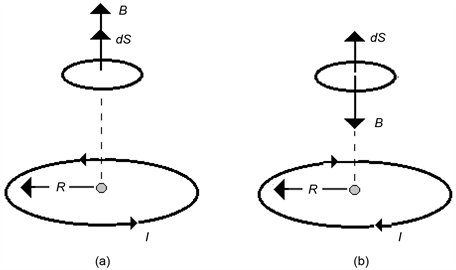
Figure A-2. Vectors B and dS: (a) In the same direction; (b) In opposite directions.
(A.8)
After some algebraic manipulation, one obtains the following expression for the axially-directed magnetic force between the coaxial coils,
(A.9)