Journal of Electromagnetic Analysis and Applications
Vol.07 No.03(2015), Article ID:54852,13 pages
10.4236/jemaa.2015.73009
Integrated and Explicit Boundary Conditions of Electromagnetic Fields at Arbitrary Interfaces between Two Anisotropic Media
Bing Zhou1, Graham Heinson2, Aixa Rivera-Rios2
1Petroleum Geosciences, The Petroleum Institute, Abu Dhabi, UAE
2Geology and Geophysics, The University of Adelaide, Adelaide, Australia
Email: bizhou@pi.ac.ae, graham.heinson@adelaide.edu.au, aixa-rivera-rios@adelaide.edu.au
Copyright © 2015 by authors and Scientific Research Publishing Inc.
This work is licensed under the Creative Commons Attribution International License (CC BY).
http://creativecommons.org/licenses/by/4.0/


Received 3 March 2015; accepted 16 March 2015; published 19 March 2015
ABSTRACT
This paper derives two new integrated and explicit boundary conditions, named the “explicit nor- mal version” and “explicit tangential versions” respectively for electromagnetic fields at an arbitrary interface between two anisotropic media. The new versions combine two implicit boundary equations into a single explicit matrix formula and reveal the boundary values linked by a 3 × 3 matrix, which depends on the interface topography and model property tensors. We analytically demonstrate the new versions equivalent to the common implicit boundary conditions and their application to transformation of the boundary values in the boundary integral equations. We also give two synthetic examples that show recovery of the boundary values on a hill and a ridge, and highlight the advantage of the new versions of being a simpler and more straightforward method to compute the electromagnetic boundary values.
Keywords:
Electromagnetic Theory, Electromagnetism, Boubdary Condition, Electric Anisotropy

1. Introduction
The boundary conditions are often expressed in two equations?continuity of the tangential components and discontinuity of the normal components of electromagnetic field intensities  [1] . The former is yielded by applying Stokes’ law to a differential line integral on the interface between two media, and the latter is obtained by applying Gauss’ law to a differential sized cylinder surface containing a section of the interface. This gives two separate and implicit formulae that define “boundary equations” linking the boundary values of the fields in two anisotropic media. Two boundary equations are implicit functions of the interface normal
 , electric conductivity and permittivity tensors
 , or magnetic permeability tensor
 . In isotropic cases, it is not difficult to obtain the explicit formulae of the boundary values because all these tensors reduce to scalars that make the explicit solution straightforward. The difficulty is increased in applying the separate and implicit formulae to anisotropic media and arbitrary interface topography as they do not explicitly give the solutions of the boundary values, so that they must be individually or successively employed in electromagnetic field modeling. In addition, most of numerical modeling techniques, such as finite-difference, finite-element and boundary element methods approximate the boundary values with some numerical schemes, e.g. the finite-difference method often replaces the interfaces with great gradients to produce the “strong solution” of electromagnetic fields [2] . The finite-element method employs combinations of the edge-vectors to approach the field intensities so that the boundary conditions are satisfied at the sampled points [3] . However, the accuracy of the edge-vector approximation depends on the number of the samples of the edge-vectors [4] . Also, these numerical approaches cannot simultaneously produce the complete set of boundary values due to only involving one-side boundary values in the assembled linear equations, and need an explicit formula to recover another side boundary values. In order to simplify the implementation of the boundary conditions or recover whole boundary values at an interface, it is desirable to combine the two separate and implicit equations into a single integrated and explicit formula so that it can be more directly and easily applied to theoretical and numerical electromagnetic anisotropy problems.
This paper derives two new integrated and explicit versions of the boundary conditions, called the explicit “normal” and “tangential” versions respectively. They successfully combine two common implicit boundary equations into a single explicit linear matrix formula without altering their applicability to interfaces that have arbitrary topography and two anisotropic media. These new versions consistently present the boundary values of electromagnetic field intensities  linked by a 3 × 3 matrix, which can be calculated with the known interface topography
  and tensors of model electric permittivity
 , conductivity
  and magnetic permeability
 . We analytically demonstrate equivalence of the single matrix formula to two common implicit boundary equations, and show theoretical applications of the new versions to transformation of the boundary values from one-side to another in the boundary integral equation and boundary element approach. In addition, two synthetic experiments of utilizing the new versions are conducted, and show the advantage of the new versions of being a simpler and more straightforward method to recover the whole boundary values at arbitrary interfaces.
2. Boundary Conditions
In the frequency-domain, electric and magnetic field intensities  in anisotropic media satisfy Maxwell’s equations [5]
 (1)
(1)
where  and
and  represent the external magnetic and electric current sources supplied by human or natural existence, and
  is the complex-valued tensor defined by:
 (2)
(2)
Here,  represents an angular frequency and
  are three tensors of magnetic permeability, electric conductivity and permittivity. The complex-valued conductivity tensor
  implies that the electric current density
  consists of the conduction
  and displacement
  current densities. In this paper,
  or
or  are simply called the model property tensors because they define the electromagnetic properties of media. In isotropic cases, the model property tensors
  or
or  are scalars, i.e.
  or
or . In general, the field intensities
 , model property tensors
  or scalars
 , and external current sources
  are functions of the spatial coordinates
 .
.
Applying Equation (1) and its zero-divergences  and
and  to a closed differential line integral and surface integral of a differential sized cylinder surface that contains a section of the interface between two media, respectively [1] , the following boundary conditions of the electric and magnetic field intensities are obtained:
 (3)
(3)
 (4)
(4)
Here, the scalar quantities  and
and  are the normal components of the net external current densities at the interface:
 (5)
(5)
The superscripts “−” and “+” stand for the boundary values on the two sides of the interface, and  is a unit normal of the interface (see Figure 1).
In order to remove computational singularities (infinite value) of the external point sources  and
and , the field intensities are often expressed in two portions [2] [3] [6] , i.e.
 , where
  are the primary fields generated by
  and
and  in a reference model given by
 , and
, and  are the secondary fields governed by the following equations obtained by substitution of the field decomposition into Equation (1):
 (6)
(6)
These equations demonstrate that the source terms of the secondary fields are  and
and  instead of
  and
and , where
 , Similarly, Applying Equation (6) and its zero diver-
gences to an interface of two media, and appointing ,
,  or
or ,
,  in the cases of
  or
or  respectively, the following boundary conditions of the secondary fields are obtained:
 (7)
(7)
 (8)
(8)
Here,  and
and . Equations (7) and (8) are also yielded by substituting
  and
and  into Equations (3) and (4) respectively, and then applying the same boundary conditions to the primary fields. Equations (3) and (4) or Equations (7) and (8) are general and applicable to any interface between two media. Here, we named these boundary conditions as the “implicit boundary equations” because they consist of two separate and implicit equations that involve the boundary values of the field intensities
 , unit normal
  of an interface and model property tensors
 . By comparing Equation (3) with (4), or Equation (7) with (8), the similarities of the boundary conditions of magnetic fields to electric fields are observed. It is shown that the boundary conditions of magnetic fields can be obtained by simply replacing the electric field symbols
  with the magnetic field symbols
 . Therefore, derivations below will only deal with electric field whose result can be easily extended to magnetic field by the symbol replacements.
3. Explicit Normal Version
Equation (3) can be rewritten in the following matrix form
 , (9)
, (9)
where the vectors  and
and  are defined by
  and
and  respectively, and the matrices
  are given by:
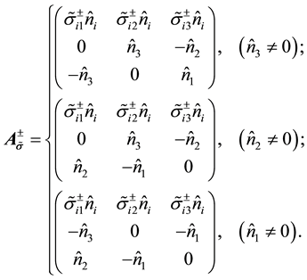 (10)
(10)
Here, the summation convention over the double subscripts  has been applied, and the redundant row arising from curl calculation has been removed in three cases. Accordingly, the determinant of the matrix cannot be zero
 , therefore, the matrix
  is invertible and its inverse matrix can be calculated by linear algebra:
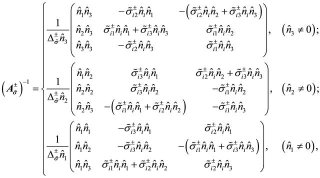 (11)
(11)
where
 . (12)
Multiplying  to Equation (9) gives
 (13)
(13)
where
 , (14a)
or
 (14b)
(14b)
Here,  is the Kronecker delta symbol. The above equation shows that the three cases given in Equations (10) and (11) are unnecessary in the matrix
 . In this paper, the matrix
  is called the boundary matrix because it is a function of the boundary conductivity tensors
  and the unit normal
  of the interface, and links the two boundary values of the field intensities. With the known interface normal
  and conductivity tensors
 , Equation (13) directly give the solution of the boundary values and successfully combines two implicit boundary equations into a single explicit linear matrix formula. This integrated and explicit form of the boundary conditions is advantageous to application without altering its applicability to any interface between two media. Therefore, Equation (13) is termed the “explicit normal versions” of the boundary conditions.
Substituting  into Equation (13) and then applying the same boundary conditions to the primary fields
  in the reference conductivity model:
 ,
,  or
or ,
,  , the integrated and explicit boundary conditions of the secondary electric fields are obtained:
 (15)
(15)
This equation corresponds to Equation (7) but explicitly gives the boundary values of the secondary fields. It achieves transformation of the boundary values at an interface.
The explicit boundary conditions for magnetic fields can be obtained by replacing the electric symbols  with the magnetic symbols
  in Equations (13) and (15), i.e.
 (16)
(16)
 (17)
(17)
From these explicit normal versions, it is apparent that the boundary matrices  are crucial in
solving the boundary values of the field intensities. With given model property tensors  and interface
normal , the boundary values can be directly calculated through the boundary matrix. This mathematical merit is not possessed by the implicit boundary equations given in the previous section when dealing with the arbitrary interface between two anisotropic rocks.
In isotropic media,  and
and , and Equation (14b) is changed into
 . (18)
This indicates that if there is no difference in model properties, the boundary matrix becomes a unit matrix  due to
 . It indicates that the field intensity maintains its continuity when the net external current source is zero at the interface
 .
.
At the air-earth interface, we have  (pure imaginary value) and
 , the boundary matrix Equation (14b) becomes
 (19)
(19)
Specifically, if the electric permittivity of the earth is the same as air, i.e. , Equation (19) is reduced to
 (20)
(20)
It indicates that if the electric field  is real
  and the net external current source continues at the interface, then the real and imaginary boundary values on the “+” side are given by
  and
and  respectively. This shows that the imaginary values of the field intensity on the “+” side are not zero cross the interface.
4. Explicit Tangential Version
In contrast to the implicit formulae given by Equations (3) and (6), the explicit normal versions of the boundary conditions, e.g. Equations (13) and (18), do not directly indicate continuity of the tangential components of electromagnetic field intensities  at an interface due to absence of the tangential vectors of an interface. In order to overcome this weakness, three perpendicular interface vectors
  are introduced at a point of the interface (see Figure 1):
 (21)
(21)
Here, the angles  are calculated by
 (22)
(22)
where  defines topography of an arbitrary interface. According to spline theory [7] ,
  may be approached by a 2-D spline interpolation:
 . (23)
The coefficients  are defined in the subdomain
  and determined by the known regularly-gridded or scattered samples of
 . According to the spline theory, Equation (23) guarantees the continuity of the interface vectors
  at every point of the interface. Equations (21) and (22) indicate that the interface vectors
  change with the interface topography
 . If it is flat
 , then the interface vectors
  become the Cartesian vectors
  or
or , which are the constant directions of the x-, y- and z-axis. Consequently, the electromagnetic field intensities may be expressed by either the Cartesian or interface-vector forms, i.e.
 . (24)
Therefore, Equation (3) can be rewritten in the following forms:
 (25)
(25)
Combining these two equations yields
 , (26)
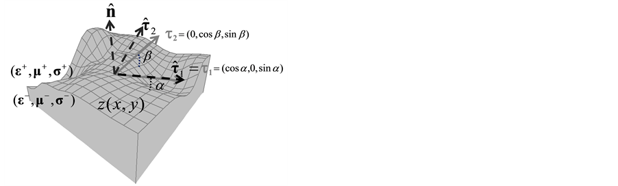
Figure 1. Illustration of three perpendicular vectors  at a point of an interface
 .
.  and
and  are the slope vectors of the interface and are employed to compute the normal
  of the interface. The perpendicular tangential vectors
  are obtained by assigning
  and the cross product
 .
.
where
 (27)
(27)
Substituting Equation (26) into Equation (24) results in
 (28)
(28)
and
 (29)
(29)
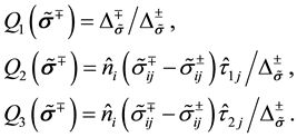
where
 . (30)
Upon comparing Equations (29) and (30) with Equations (13) and (14), it is apparent that Equation (29) displays the same explicit linear matrix form as Equation (13) but with different boundary matrices ; the boundary matrix
  given by Equation (30) involves two tangential vectors
 , whereas the previous matrix
  given by Equation (14) does not. Therefore, it can be deduced that Equation (30) is another form of Equation (14), and given the term “explicit tangential versions” of the boundary conditions to distinguish from the explicit normal versions.
Similarly, substituting  into Equation (29) and then applying the boundary conditions
 in the reference model tensor
 ,
,  or
or ,
,  , the following explicit tangential versions of the boundary conditions are obtained:
 (31)
(31)
Equations (29) and (31) can be changed for magnetic field intensity by symbol replacements:
 (32)
(32)
 (33)
(33)
These equations correspond to Equations (4) and (8), or Equations (16) and (17).
At an isotropic interface,  and
and . Thus, Equation (30) can be simplified to
 , (34)
At the air-earth interface, Equation (30) becomes
 , (35)
and if the media possesses the same electric permittivity as air, i.e. , Equation (35) is changed into
 . (36)
5. Equivalence of the Different Version
The two integrated and explicit boundary conditions formulated above demonstrate a matrix  that can be calculated by either Equation (14) or Equation (30). Although the two versions are derived from the same implicit formulae, e.g. Equations (3) and (7), the boundary matrices
  appear to differ. From a mathematical perspective, the different versions, i.e. explicit normal and tangential versions, as well the original implicit equations should be equivalent to each other because of uniqueness of the boundary values.
Multiplying the matrix  to Equation (13), and then applying the factorization of the boundary matrix
 , the matrix form of Equation (3) is obtained from Equation (13):
 (37)
(37)
Similarly, Equations (15), (16) and (17) can be changed into Equations (7), (4) and (8) respectively. These formulations show that the explicit normal versions are equivalent to two common implicit boundary equations.
Applying the perpendicular properties of the interface vectors to Equation (30), e.g. ,
,  and
and , the following equations are obtained:
 (38)
(38)
Substituting these identities into Equation (29) yields
 (39)
(39)
These equations indicate continuity of the tangential components and discontinuity of the normal components of the electric field intensities. It proves that the explicit tangential versions are also equivalent to two common implicit boundary conditions.
Note that the three interface vectors given by Equation (21) satisfy the following equation
 . (40)
Accordingly, equation (30) may be rewritten as follow
 (41)
(41)
which is the same as Equation (14b). Similarly, substituting Equation (40) for Equations (34), (35) and (36) respectively, they become Equations (18), (19) and (20). Therefore, the explicit tangential versions are equivalent to the explicit normal versions and vice versa as Equation (41) are reversible. Specifically, when the two media have the same electric permittivity , i.e.
 , Equation (41) is changed into
 (42)
(42)
This shows the small imaginary value  when a low frequency is considered.
6. Transformation of Boundary Values
The boundary element theory has shown that if there is not any external current source  and
and  in a homogeneous medium, the electromagnetic field intensities
  in the medium domain
  may be expressed by the following boundary integral [8] :
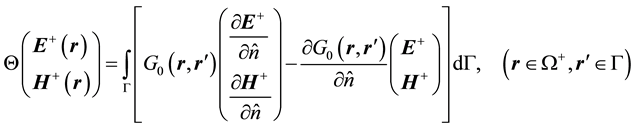 . (43)
Here,  is the Greens function of the homogeneous medium,
  takes the values of 1.0, 0.5 and
  responses to
 ,
,  (smooth) and
  (not smooth) respectively, and
  is the corner angle at
 . This equation indicates that calculation of the electromagnetic field intensities
  in the homogeneous medium require not only the boundary values of the field intensities
  but also the normal derivatives
 . The boundary element method based on Equation (43) [8] [9] offers a tool to find the boundary values
  or
or  with the known field intensities
  or normal derivatives
 . Unfortunately, in most of electromagnetic modeling cases, neither the boundary values of the field intensities
  nor the normal derivatives
  are known. However, if the field intensities
  in the connected domain
  are given or going to be solved, the normal derivatives
  at the interface can be calculated by numerical differentiations with the known or solved field intensities
 . In this case, application of Equation (43) needs transformations of the boundary values from
  to
to . Apparently, the integrated and explicit boundary conditions presented in the previous sections are directly applicable to these transformations, e.g. substituting Equations (13) and (16) for the second term of the right-hand-side surface integral of Equation (43) achieves the transformation of the boundary values
  into
into . For transforming the normal derivatives
  into
into , one may follow the same methodology as described in the previous sections and obtain the integrated and explicit boundary conditions of the normal derivatives.
We calculate  on both sides of Equation (1) and obtain
 (44)
(44)
which give zero divergences
 (45)
(45)
Applying Equations (44) and (45) to an interface of two anisotropic media, we obtain the boundary conditions of the partial derivatives:
 (46)
(46)
and
 (47)
(47)
Therefore, we have the following integrated and explicit versions of Equations (46) and (47):
 , (48)
 , (49)
where the components of matrices  and
and  are given by
 (50)
(50)
Applying Equations (13), (16), (48) and (49) for Equation (43), one can fulfill the transformations of the boundary values from the domain  into
into , in which the field intensities
  are going to be solved and the normal derivatives
  can be calculated with the given interface topography
  and its nearby field intensities
 . Particularly, after achieving the transformations of the boundary values, the boundary integral
  in Equation (43) can be approached by the boundary element method [9] that results in
  (total points of the interface) linear equations of the field intensity
  or
or . These equations are considered as “the boundary equations” of the field intensities
  and independently complementary to the linear equations yielded by other numerical approach applied to the domain
 , e.g. finite-difference or finite-element method. Therefore, the numerical computations of the field intensities
  are implemented only in the domain
  and have nothing relating to
 , so that the computational dimensions are significantly reduced. These developments of hybrid methods are beyond the topic of this paper and will be given in our future articles.
7. Synthetic Examples
In order to demonstrate possible applications of the integrated and explicit versions of the boundary conditions, synthetic experiments of a hill and a ridge model have been conducted (see Figure 2 and Figure 4). These models may represent the Earth’s surface, or seafloors, or subsurface interfaces of rocks. The synthetic experiments were only carried out using electric fields  with the explicit normal versions due to the similarity between magnetic fields
  and electric fields
 , and the equivalence of the two explicit versions. In these experiments, the frequency of 0.1 Hz and an external plane-wave source at infinity were considered
 , and the hill and ridge interfaces were approximated by Equation (23) using regularly-gridded samples of the interface topographies. Above the interface, the conductivity tensor
  was assigned to the air
  and an anisotropic medium
  respectively. Below the interface, a different anisotropic medium was applied
 . These two media have the same electric permittivity as air. In addition, we assumed the boundary values of the electric field intensity
  in the air-domain are known, e.g.
 ,
,  , which represents the observed data on the Earth’s surface or seafloor from a practical measurement [10] , or the numerical solution from the boundary element method [8] [9] . The new integrated and explicit versions enable us to directly recover the boundary values
  under the ground or seafloor. It is possible to combine the transformed boundary values with other numerical method in
  and perform the forward modeling or tomographic inversion without the air or seawater domain.
Figure 2 displays the synthetic results at the air-earth interface of a hill. Three components of the boundary values  are plotted and show discontinuities throughout the vertical components
 , and continuity in the horizontal components
  at the flat portions of the interface due to
  and
and . Discontinuity of
  in the hill area arises when
  and
and . It also shows that the imaginary parts
  are very small
  due to the low frequency (0.1 Hz) and same electric permittivity
  of the two media. Therefore, these imaginary parts are often ignored in most magnetotelluric measurements [1] .
Figure 3 demonstrates three components of the electric current density , whose real
  and imaginary values
  display the conduction and displacement current densities respectively. These diagrams indicate that the conduction current density disappears in air
  due to zero
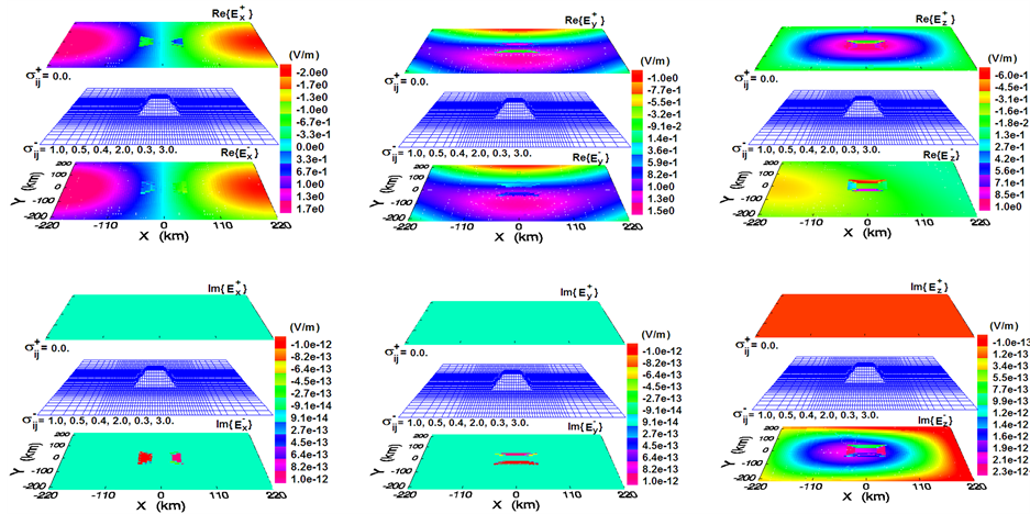
Figure 2. Synthetic results of electric fields 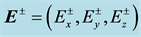 at the air-earth interface that has a hill topography and anisotropic ground. The images over and under the surface give the boundary values
 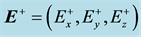 and
and  computed by the explicit normal versions of the boundary conditions.
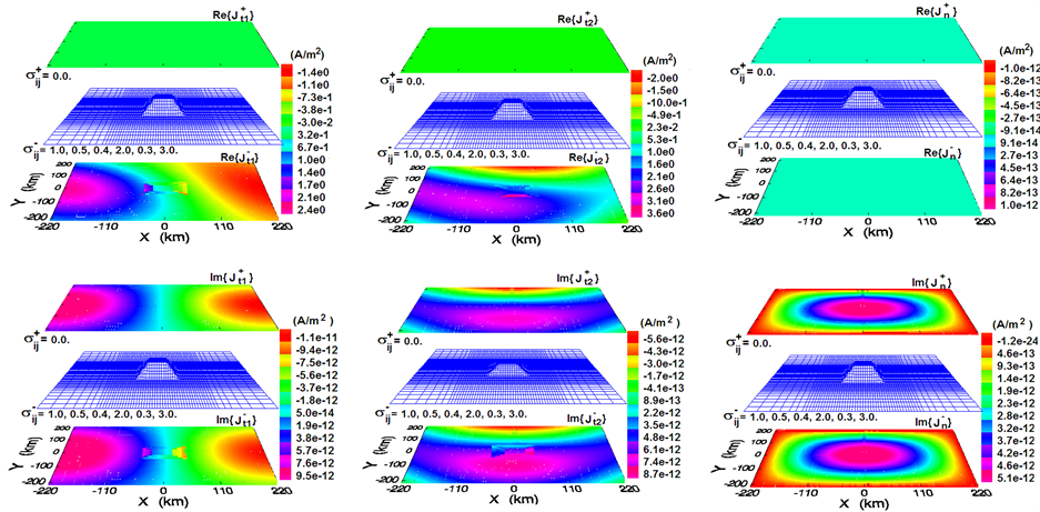
Figure 3. Synthetic results of electric current density  at the air-earth interface that has a hill topography and anisotropic ground. The images over and under the surface are the boundary values
  and
and  computed by the explicit normal version of the boundary conditions.
conductivity  and displacement current density occurs
  because of non-zero electric permittivity
 , whilst the normal total current densities remain unchanged
  and the tangential total current densities vary
 . These characteristics are predictable from the implicit boundary equations.
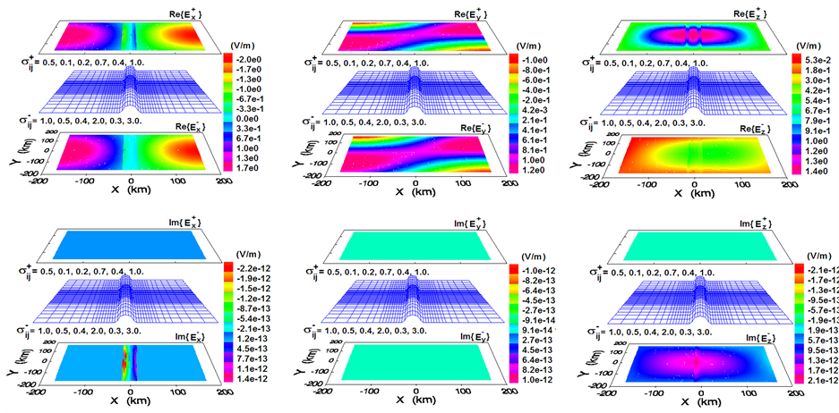
Figure 4. Synthetic results of electric fields  at a ridge interface between two anisotropic rocks. The images over and under the surface give the boundary values
  and
and 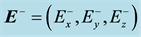 computed by the explicit normal version of the boundary conditions.
Figure 4 demonstrates the synthetic results of a ridge interface that connects two anisotropic media. Similar characteristics to those in Figure 2 are again observed, including discontinuities throughout the vertical components , continuity in the x-components
  except in the ridge area where
 , and continuity in the y- component
  in all areas due to
  (see the middle panel in Figure 4). Figure 5 demonstrates three components of the electric current density
 , which indicate that the conduction and displacement current densities exist in the two media, and the tangential current densities
  differ from
  because of two different conductivities, but the normal currents
  remain the same regardless of the interface topography.
8. Conclusions
Two new integrated and explicit boundary conditions, termed the “normal” and “tangential” versions, have been presented in this paper for electromagnetic fields at an arbitrary interface between two anisotropic media. These two versions both achieve combination of two implicit boundary equations into a single explicit linear matrix form, and consistently reveal that the boundary values are linked by a 3 × 3 boundary matrix dependent on the interface topography and electric conductivity or magnetic permeability tensors of the media. The normal version shows that the boundary matrix is calculated with the known normal of the interface and model property tensors; while the tangential version indicates that the boundary matrix requires two perpendicular tangential vectors besides the normal of the interface. However, despite these differences, the mathematical equivalence of the two new versions to each other, as well as to the standard implicit boundary conditions is demonstrated. With known normal  of an interface, the explicit normal version is more compact and efficient compared to the explicit tangential version because the two perpendicular tangential vectors
  are not required. With a given interface
 , there is no difference between the two versions in computational efficiency as the tangential vectors
  and normal
  must be calculated from the interface topography function
 .
.
The synthetic examples of a hill and a ridge interface demonstrate possible applications in conversions of the boundary values, and capability of the new versions to arbitrary interfaces that may involve complex topography and anisotropic rocks. These results numerically show continuity of the tangential components and discontinuities of the normal components of electromagnetic field intensities, and continuity of the normal components and discontinuities of the tangential components of electric current densities across the air-earth interface and the boundary of two anisotropic rocks. These synthetic examples also demonstrate that the boundary values of the
Figure 5. Synthetic results of electric current density  at a ridge interface between two anisotropic rocks. The images over and under the surface show the boundary values
  and
and  respectively, computed by the explicit version of the boundary conditions.
field intensities may change with alterations in topography of the interface, electric conductivity and permittivity tensors, or magnetic permeability tensors. It is shown that with help of the new integrated and explicit versions, the unknown boundary values can be obtained by simply multiplying a boundary matrix with the known boundary values. Therefore, it provides a more straightforward and easier method to transform the boundary values from one domain to another. It is greatly helpful to not only extrapolation of electromagnetic fields with the boundary element approach, but also combination of the boundary element approach with other numerical methods, such as finite-difference, finite-element and integral equation method, because the boundary element approach with the transformed boundary values can offer complementary linear equations to these numerical methods, so that the numerical computations remain in the interesting model domain and the computational dimensions are significantly reduced.
Acknowledgements
This work was supported by a Discovery Project (DP1093110) of the Australia Research Council. The authors thank Mr. Craig Patten for his assistance in using high-performance computing facility at e Research SA in Australia.
References
- Weaver, J.T. (1995) Mathematic Methods for Geo-Electromagnetic Induction. Research Studies Press Ltd., Taunton, Somerset.
- Key, K. and Weiss, C. (2006) Adaptive Finite-Element Modeling Using Unstructured Grids: The 2D Magnetotelluirc Example. Geophysics, 71, G291-G299. http://dx.doi.org/10.1190/1.2348091
- Mukheriee, S. and Everett, M. (2011) 3D Controlled-Source Electromagnetic Edge-Based Finite Element Modeling of Conductive and Permeable Heterogeneities. Geophysics, 76, F215-F226. http://dx.doi.org/10.1190/1.3571045
- Axia, R. (2014) Multi-Order Hexahedral Vector Finite Element Method for 3-D MT Modeling, Including Anisotropy and Complex Geometry. PhD Thesis, Adelaide University, Adelaide.
- Thide, B. (2004) Electromagnetic Field Theory. Upsilon Books, Communa AB, Uppsala.
- Zhdanov, M.S., Varentsov, I.M., Waever, J.T., Golubev, N.G. and Krylov, V.A. (1997) Methods for Modeling Electromagnetic Fields Results from COMMEMI―The International Project on the Comparison of Modeling Methods for Electromagnetic Induction. Journal of Applied Geophysics, 37, 133-271. http://dx.doi.org/10.1016/S0926-9851(97)00013-X
- Helmuth, S. (1995) Two Dimensional Spline Interpolation Algorithms. A. K. Peter Ltd, Wellesley.
- Brebbia, C.A. and Dominguez, J. (1992) Boundary Elements: An Introductory Course. Computational Mechanics Publications, Boston.
- Beer, G., Smith, I.M. and Duenser, C. (2008) The Boundary Element Method with Programming for Engineering and Scientists. Springer Wien, New York.
- Everett, M.E. and Constable, S. (1999) Electric Dipole Fields over an Anisotropic Seafloor: Theory and Application to the Structure of 40Ma Pacific Ocean Lithosphere. Geophysical Journal International, 136, 41-56. http://dx.doi.org/10.1046/j.1365-246X.1999.00725.x