Journal of Electromagnetic Analysis and Applications
Vol.4 No.7(2012), Article ID:21262,12 pages DOI:10.4236/jemaa.2012.47041
The Modeling of 2D Controlled Source Audio Magnetotelluric (CSAMT) Responses Using Finite Element Method
![]()
1Physics of Earth and Complex System, Faculty of Math and Natural Sciences, Institut Teknologi, Bandung, Indonesia; 2Geophysics, Physics Department, Universitas Padjadjaran, Bandung, Indonesia; 3Applied Geology, Faculty of Earth Science and Technology, Institut Teknologi Bandung, Indonesia.
Email: imran.hilman@phys.unpad.ac.id
Received May 1st, 2012; revised June 3rd, 2012; accepted June 15th, 2012
Keywords: EM Modeling; CSAMT; Finite Element Method
ABSTRACT
This paper presents the modeling of 2D CSAMT responses generated by horizontal electric dipole using the separation of primary and secondary field technique. The primary field is calculated using 1D analytical solution for homogeneous earth and it is used to calculate the secondary electric field in the inhomogeneous Helmholtz Equation. Calculation of Helmholtz Equation is carried out using the finite element method. Validation of this modeling is conducted by comparison of numerical results with 1D analytical response for the case of homogeneous and layered earth. The comparison of CSAMT responses are also provided for 2D cases of vertical contact and anomalous conductive body with the 2D magnetotelluric (MT) responses. The results of this study are expected to provide better interpretation of the 2D CSAMT data.
1. Introduction
The CSAMT method was introduced by Goldstein and Strangway [1] who performed the method in the field with massive sulphide anomaly. Sandberg and Hohmann [2] have successfully applied the method in geothermal field, and suggested that the plane wave assumption is valid at the receiver-transmitter distance greater than five skin depth. CSAMT applications in geothermal have also been studied by Wannamaker [3,4]. In petroleum application, Ostrander et al. [5], have performed a mapping of electric field anomaly in oil field using CSAMT. Other applications in petroleum exploration were carried out by Hughes and Carlson [6], which performed the mapping of structure in oil field. Bartel and Jacobson [7] used the method to determine the depth and nature of volcanic thermal anomalies using the electric properties, and suggested the correction of CSAMT data in order to fulfill the plane wave assumption.
In general, the response function of CSAMT modeling is based on assumption that the source of electromagnetic field (EM) used is in the form of the plane wave. The assumption can be fulfilled only when the measurement of CSAMT data is conducted on the radiation zone, which is around five times the “skin depth” of EM wave under consideration [2,3,8]. In practice, the assumption often can not be fulfilled due to various constraints, such as the limitations of resources and the complexity of the local topography. This conditions makes the measurement cannot be conducted on the radiation zone. As the consequence, CSAMT data should be corrected to eliminate the influence of “non-plane wave effects” [7,9]. However, the correction is not possible if the influence is large enough. Thus it is very important to develop the full solution modeling of CSAMT responses.
The full solution for CSAMT 1D has been widely developed and can be found in literatures such as Kauffman-Keller [10], Ward and Hohmann [11] and Singh and Mogi [12]. The 1D layered earth structure can be used to interpret the structure like sediments, where the variation of conductivity depends only on depth. However, the earth structure is complex and has variation of conductivity in both 2D and 3D. Thus the full solution for 2D and 3D CSAMT responses needs to be improved.
Modeling of EM in both 2D and 3D have widely developed since decades ago. Usually the calculation of 3D EM source in 2D and 3D are carried out by solving the secondary field caused by anomalous bodies, using the 1D analytical solution as the primary field. Stoyer and Greenfield formulated the excitation of 3D source in a 2D model using finite difference method to solve the second order differential equation for the secondary fields Ex and Hx, a pair of EM field with orientation parallel to geological strike [13]. The calculation of seconddary field using finite element method was carried out by Unsworth et al., which studied the EM responses generated by finite electric dipole in marine exploration [14]. However, as stated by Mitsuhata, the conventional scheme using the secondary field calculation is not effective for complex structures, and he presented the uses of pseudo-delta function to distribute the current source without the separation of primary and secondary field [15]. Li and Key applied the adaptive grid element for the case of Controlled Source EM in marine applications [16]. Some of 3D EM modeling were carried out by Streich who developed the Finite Difference Frequency Domain (FDFD) scheme for marine applications [17].
The use of integral equation method of EM modeling can be found in many literatures, such as Lee and Morrison [18], which used the integral equation for modeling the EM response due to excitation of horizontal magnetic dipole source. Boschetto and Hohmann [19] describe the CSAMT response due to scattering of 3D objects, using the volume integral equation code developed by Newman et al., [20] to calculate the transient response due to the scattering of EM 3D objects.
In this paper 2D CSAMT responses are simulated using the summation of primary and secondary field. The calculation of secondary field is performed by using the finite element method. The finite element approach used in this paper is the Ritz method, a variational method in which the boundary value problem is formulated in terms of variational expression [21].
2. The Primary Field of CSAMT Excitation
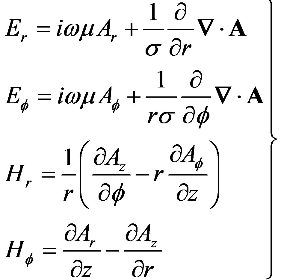
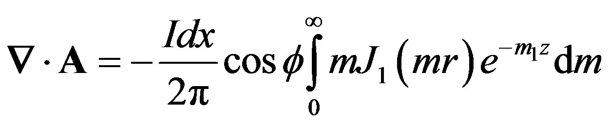
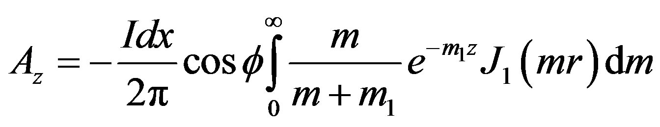
Suppose there is a homogeneous earth with conductivity of s. An electric dipole is placed on the surface with the orientation parallel to x-axis (Figure 1). The components of electric and magnetic fields in cylindrical coordinates generated by electric dipole excitation at any point below the surface is expressed as follows [10-12];
 (1)
(1)
with
 (2)
(2)
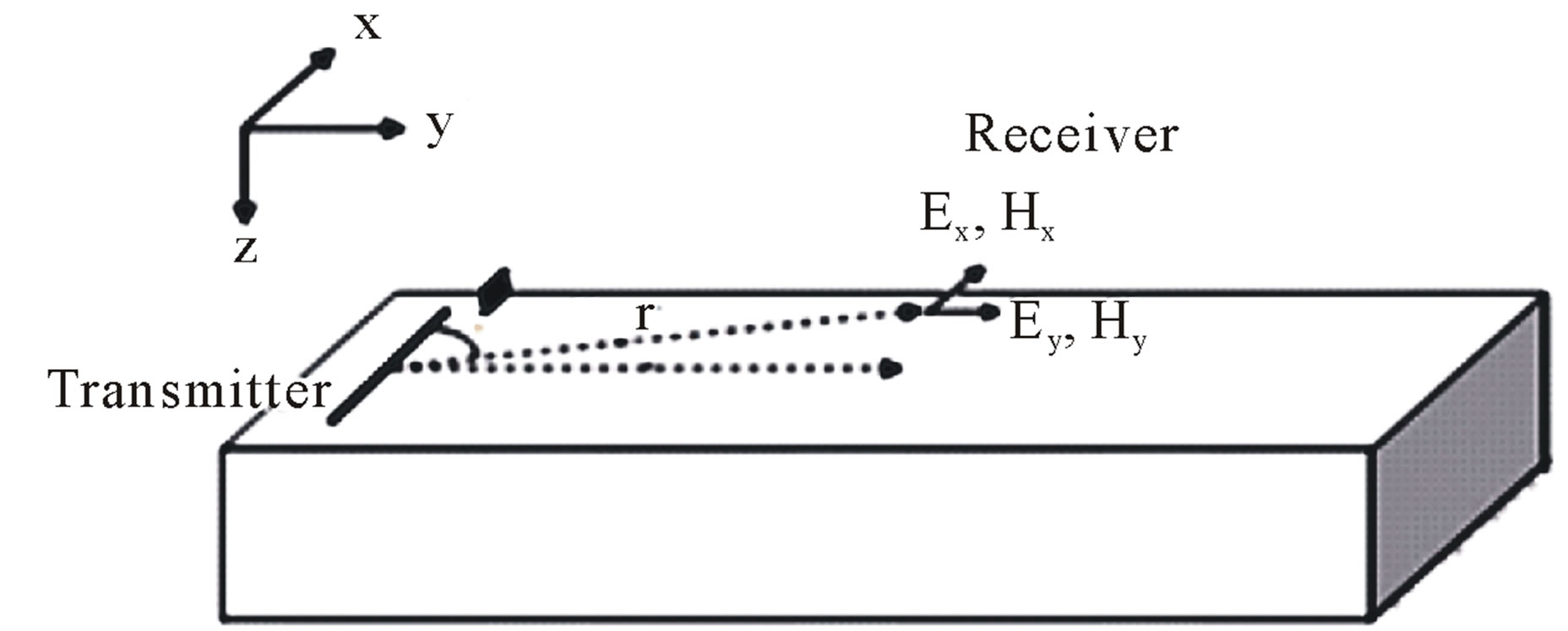
Figure 1. Field setup of CSAMT data acquisition.
 (3)
(3)
 (4)
(4)
 (5)
(5)
 (6)
(6)
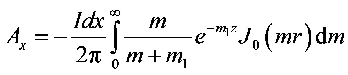
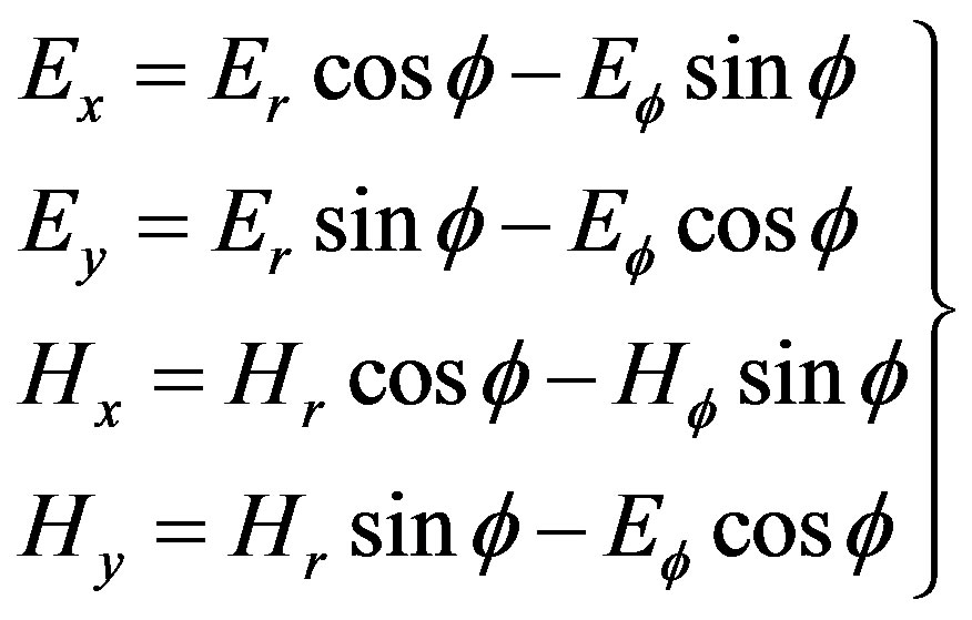
Here A is the vector potential, I expressed the current strength, dx the length of dipole, J0 and J1 are the Bessel function of order 0 and 1, w is the angular frequency, m is the magnetic permeability in vaccum and m is the wave number. Equation (1) can be used to find the field components in cartesian coordinates using the following transformation [10]:
 (7)
(7)
The field expression in Equation (7) is the primary field analytical solutions arising from the excitation of grounded electric dipole. The primary field will be used as source term in the calculation of secondary field.
The Hankel transform calculation of order 0 and 1 (i.e., the infinite integral contain Bessel function of order 0 and 1) are carried out by adaptive digital filter performed by Anderson [22,23]. Following Anderson, the Hankel transform of order n = 0,1 is defined as [22,24]:
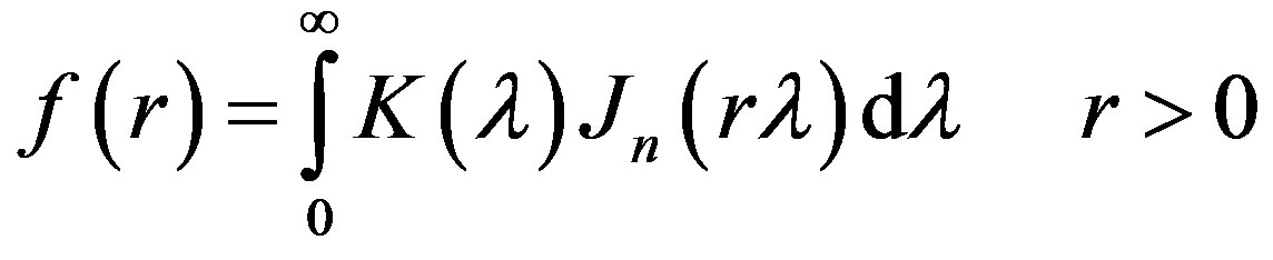 (8)
(8)
Jn is the Bessel function of first kind of n-th order.
3. Finite Element Modeling of Secondary Field
Assume the geological strike direction is on the x-axis direction as shown in Figure 1, then the inhomogeneous Helmholtz equation for electric field Ex can be expressed as [24]:
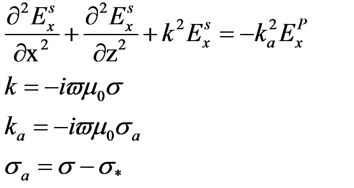 (9)
(9)
 is the primary electric field parallel to strike direction,
  is the secondary electric field generated by the presence of anomalous conductive body, ω is the frequency used, μ0 is the magnetic permeability in vacuum, σ is the total electric conductivity at a point inside the modeling domain (that is, the sum of normal conductivity without the presence of anomalous body and the anomalous body’s conductivity), σ* is the “normal” conductivity without the presence of anomalous body and σa is the conductivity of anomalous body.
The total magnetic field can be derived using curl operation to the total electric field as given by Maxwell Equation, and can be expressed as:
 (10)
(10)
The earth’s responses are usually expressed in the form of Cagniard apparent resistivity ρ and the phase of impedance , based on the relation:
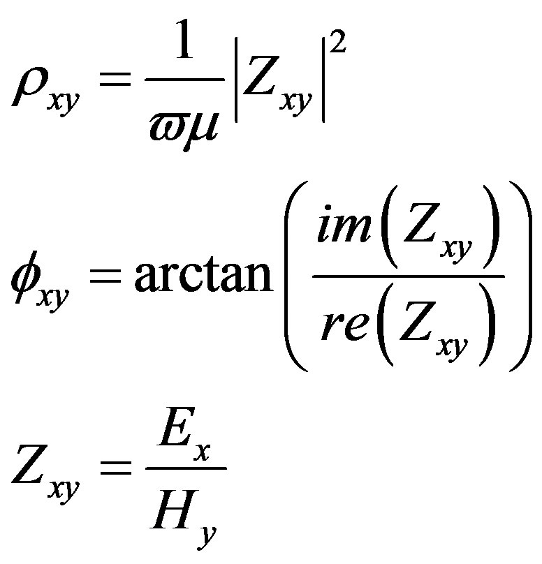 (11)
(11)
Here Zxy is the EM impedance. The subscript xy indicates that the Z component are computed by x component of electric field and y component of magnetic field.
For the case of a magnetic field with polarization parallel to the geological strike Hx, the non-homogeneous Helmholtz Equation of the secondary H field can be expressed as follows [24]:
 (12)
(12)
As in the previous case, the total magnetic field is obtained from the sum total of primary and secondary magnetic fields. The total electric field is obtained using the rotation operator to the total magnetic field
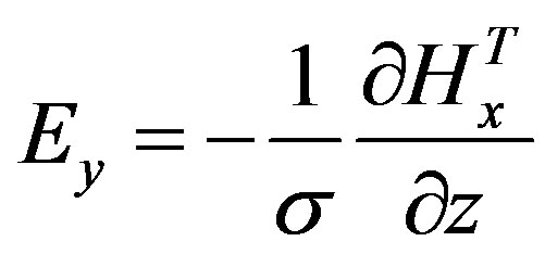 (13)
(13)
and the EM responses in the form of apparent resistivity and phase of impedance are expressed by the following equation:
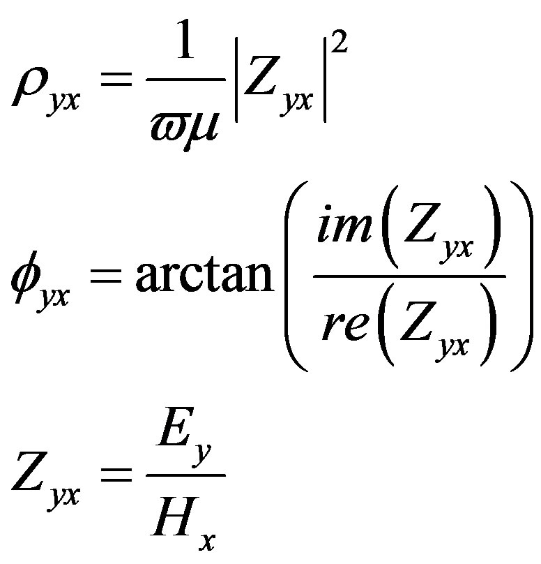 (14)
(14)
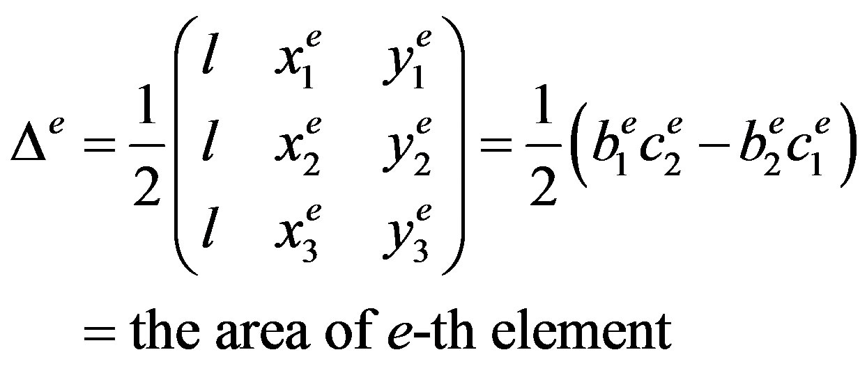
The Helmholtz Equation of secondary field, i.e. Equations (9) and (12), are the second order differential equation for the scalar field. The finite element method is used to calculate the differential Equation solution. The finite element scheme used in this modeling is the Ritz method which completely conducted by Jin [21]. The entire modeling domain is first discretized in triangular elements, using the elements as shown in Figure 2.
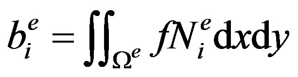
The function of EM field in each element is approximated by:
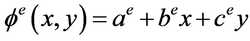 (15)
(15)
with a, b, and c are constant coefficient, and super script e is indicating the number of elements. Because there are three-nodes in the triangular element, the Equation (15) can be written as:
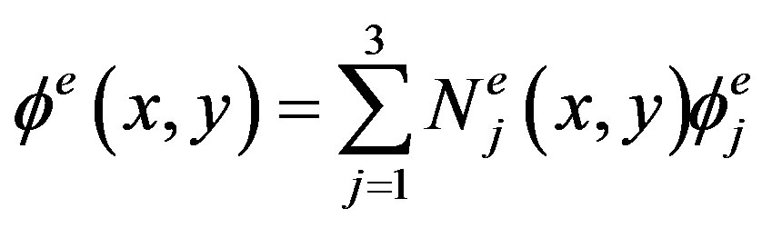 (16)
(16)
 is the interpolation function or the expansion function which has the form:
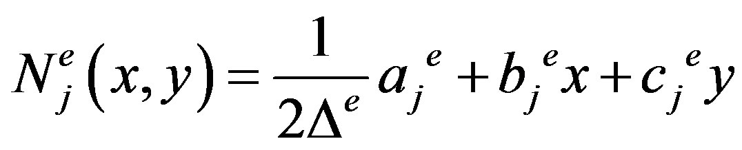 (17)
(17)
j = 1, 2, 3.
Here, the components of a, b, and c can be expressed as:
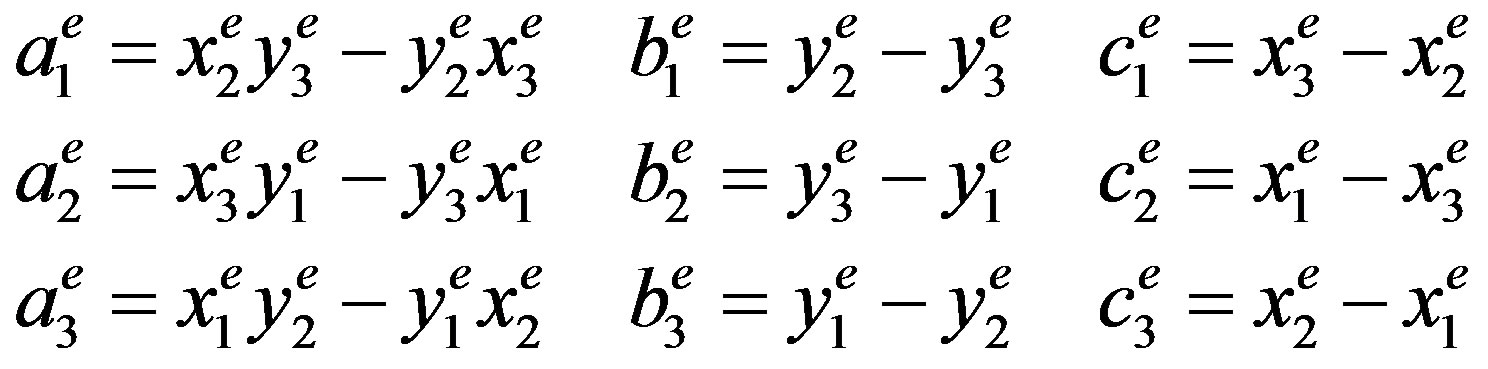 (18)
(18)
and
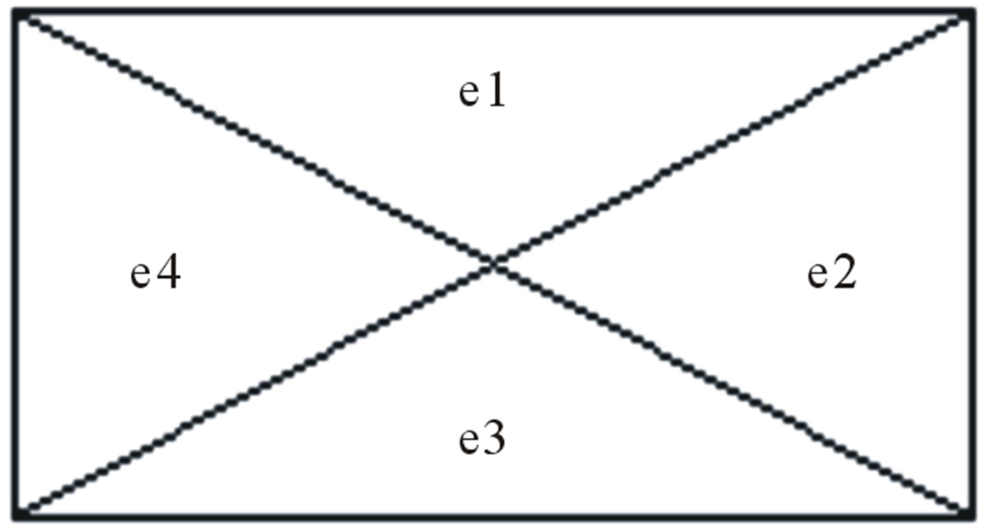
Figure 2. Triangular elements used in the modeling.
 (19)
(19)
 and
and  (j = 1,2,3) are the coordinates of j-th node. The interpolation function
 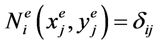 will equal to one if i = j and zero if i ≠ j.
Assume that the differential equation of secondary field problem (9) and (12), are expressed as follow:
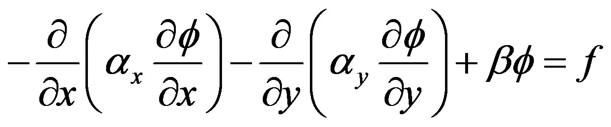 (20)
(20)
The functional can be written as
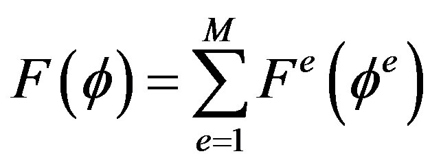 (21)
(21)
Here M denotes the total number of elements and Fe is the subfunction given by
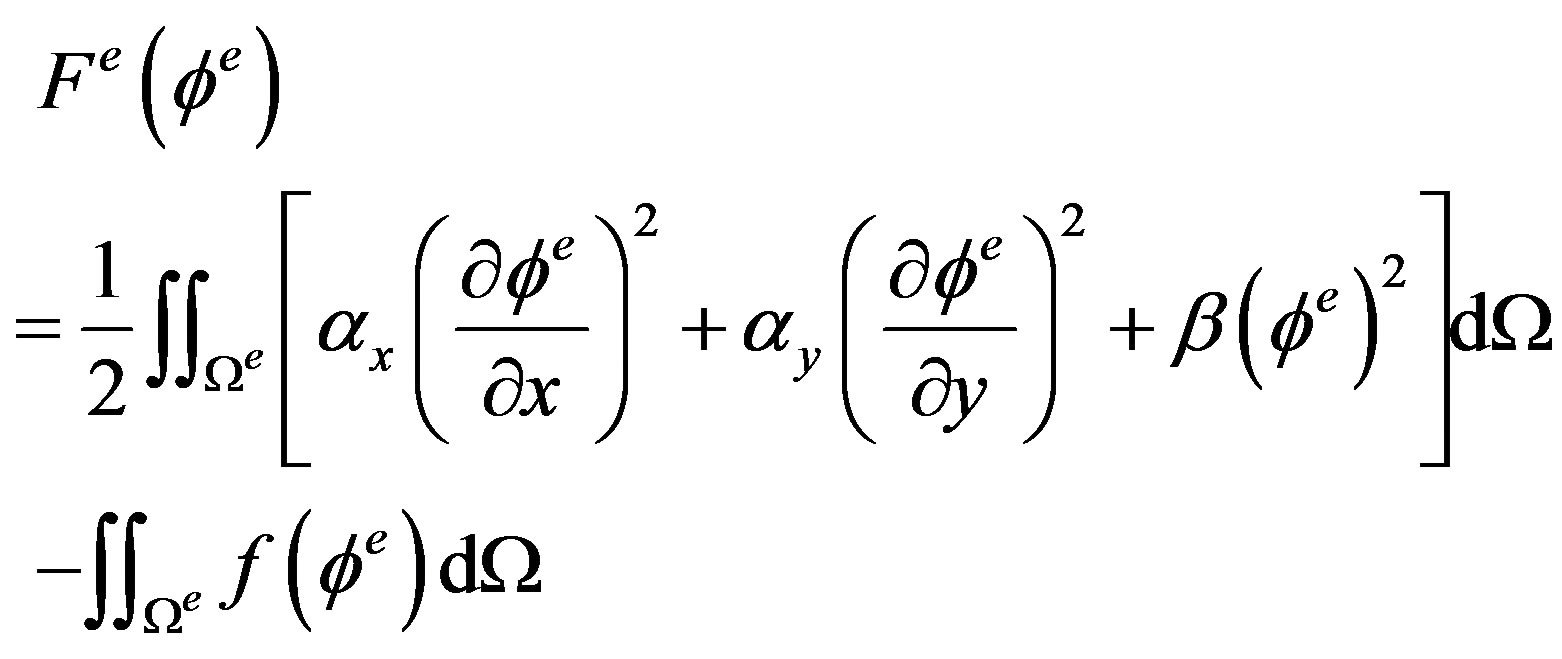 (22)
(22)
 denotes the domain of e-th element. Using the substitution of Equation (16) and differentiation of Fe with respect to
  yields,
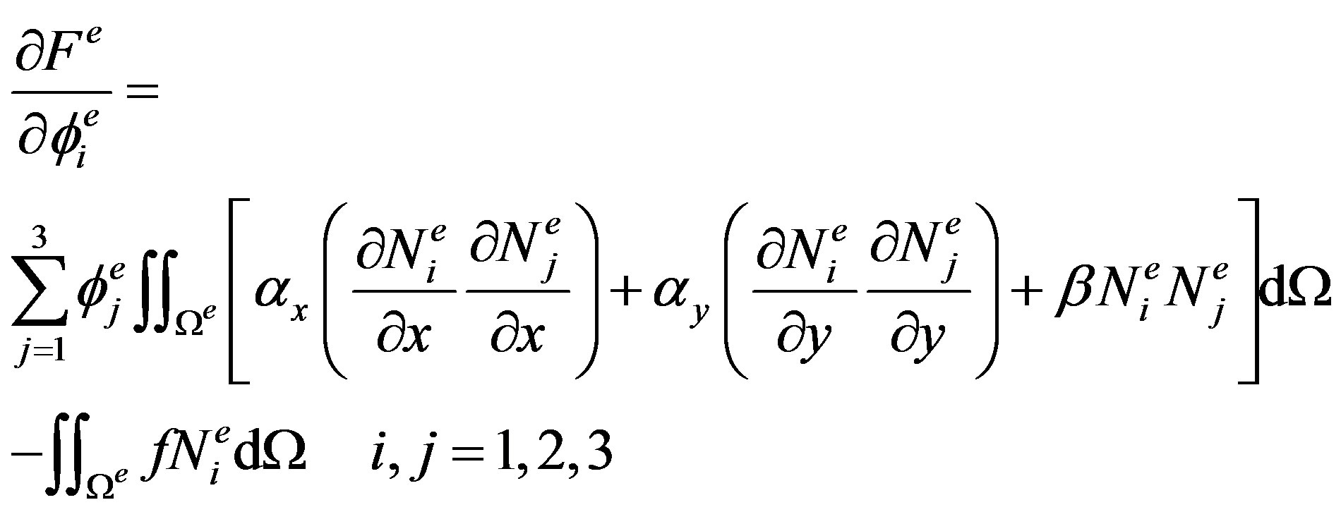 (23)
(23)
The Equation (23) can be expressed as matrix form:
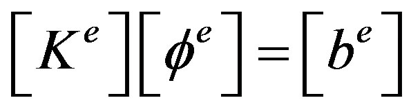 (24)
(24)
with
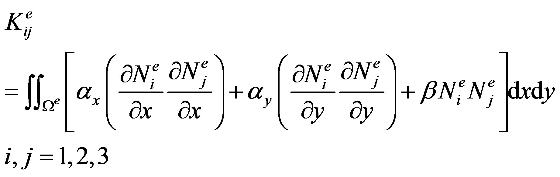
and
Equation (24) is then solved using matrix solver and yield the field’s value at the whole points inside the domain [21].
4. Results and Discussions
In this study, the transmitter is assumed parallel to the x axis as shown in Figure 3. The responses are calculated in broadside configuration, in which the sounding sites lie on the plane parallel to the transmitter’s direction. The plane is situated at the distance R to the centre of transmitter. Zonge and Hughes suggested the CSAMT measurements should be taken with the transmitter-receiver distance of 3 - 5 km. [25] Based on that assumption, the modeling is performed at plane parallel to transmitter orientation with the distance of 3 km from the centre of transmitter (Figure 3). The frequencies used in this modeling are in range of 1 Hz - 8192 Hz and has value of 2N Hz, with N is the integer from 1 to 13.
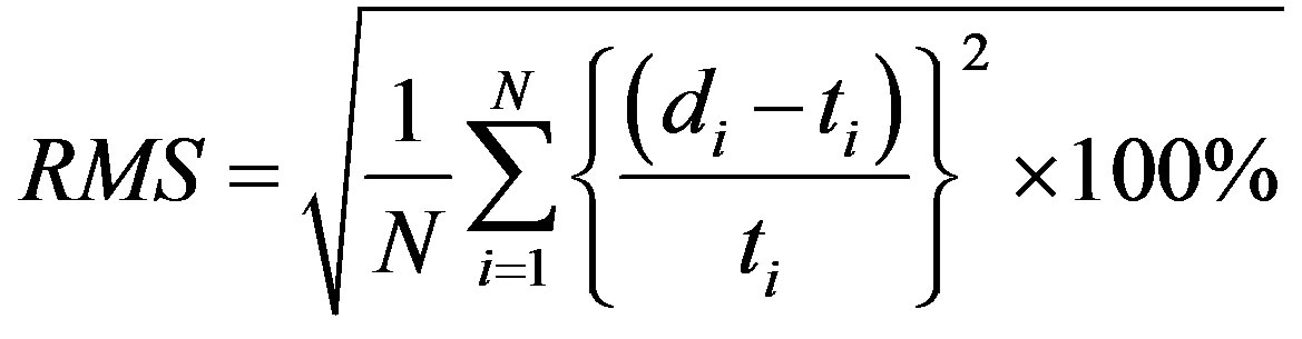
The performance of the modeling is validated by comparing the result with the responses generated by 1D analytical calculation for homogeneous and layered earth model. The source has dipole length of 1000 meters with 1 Ampere of current. Apparent resistivity and phase of impedance are calculated at one point for all frequencies. The indicator of compatibility between the analytic and numeric responses is expressed by relative RMS error, obtained by the following equation:
 (24)
(24)
di is the measurement data which obtained by 2D modeling along the line of measurement, ti the responses obtained by analytic calculation and N the number of data.
The analytic solutions of electric and magnetic fields for homogeneous earth are expressed as: [10,11]
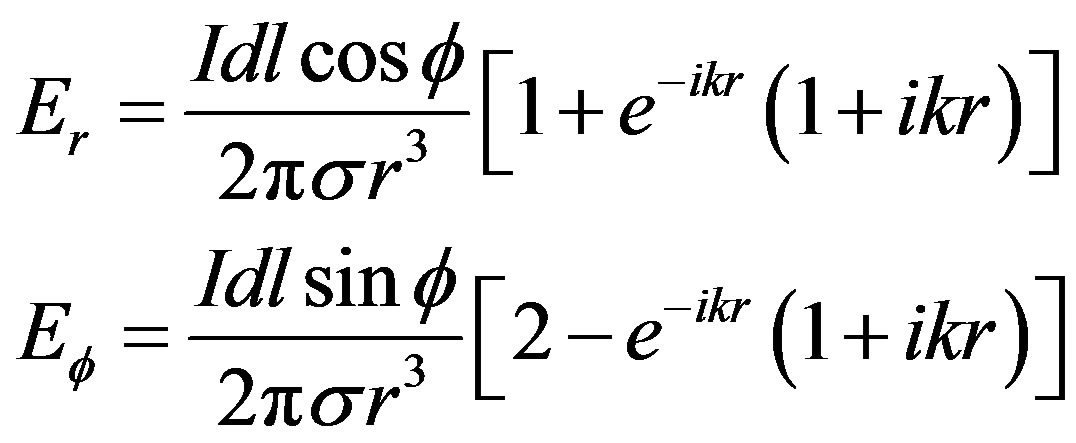 (25)
(25)
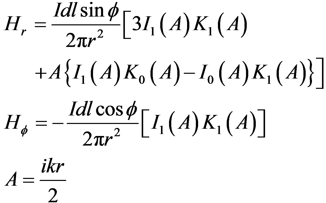 (26)
(26)
Equations (25) and (26) are then transformed using Equation (7) to obtain the electric and magnetic fields in Cartesian coordinates.
For layered earth model, numerical calculation is performed with the following steps. First, the primary field is calculated for homogeneous earth using Equation (1). The field is then used as primary field in the equation of
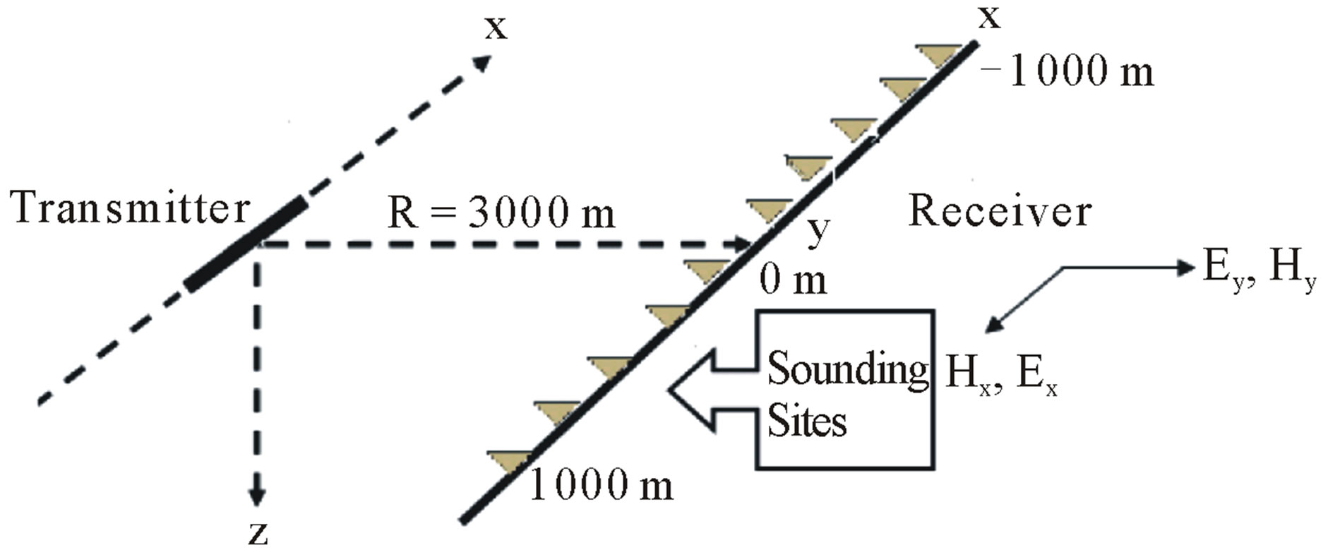
Figure 3. Broadside configuration of CSAMT data acquisition used in this modeling.
the secondary field, which occur by the scattering of anomalous layered earth. The primary and secondary field are then summed to obtain the total field, for further calculation of apparent resistivity and phase of impedance, and compared with the analytical solution by Equation (24).
For the homogeneous and three layered earth model, the sounding sites where the responses are calculated consist of three different sites: 1) –1000 meters, 2) 200 meters and 3) 1000 meters, as shown in Figure 3. The conductivity for homogeneous earth model is 100 Ohm-meters. Figure 4 shows the compatibility of modeling results with analytical solutions for homogeneous earth of xy configuration. According to Table 1, RMS errors for the xy configuration are 0.37% for apparent resistivity and 0.36% for phase of impedance, indicating good compatibility between the numerical and analytical responses. Figure 5 is clearly shows the responses of yx configuration are less close to the analytic solution. Table 1 shows RMS error of 3.5% for apparent resistivity and 2.0% for phase of impedance, indicating the error is relatively higher than the previous configuration.
The 1D layered earth model consist of three layers with resistivity of 100 Ohm-meters, 1 Ohm-meters and 10 Ohm-meters for the upper, middle and bottom layers respectively. The thicknesses of the layers are 500 meters for the first layer and 500 meters for the second layer as shown in Figure 6. The three layered earth responses are shown in Figures 7 and 8. From Table 1, the RMS error of the responses are 3.56% apparent resistivity and phase of impedance RMS error of 1.1% for xy configuration, while the configuration yx has error of 5.83% for the apparent resistivity and 0.7% for phase of impedance. As the previous model, the xy configuration shows relatively better compatibility to analytic solution than yx configuration. The layered earth model has RMS error responses higher than homogeneous models, these higher errors exist because the earth layers are treated as anomalous object in the homogeneous earth.
In general, the modeling responses in xy configuration show good agreement to analytical responses compared to the responses obtained by yx configuration, and the relative RMS error of both configurations are still in the
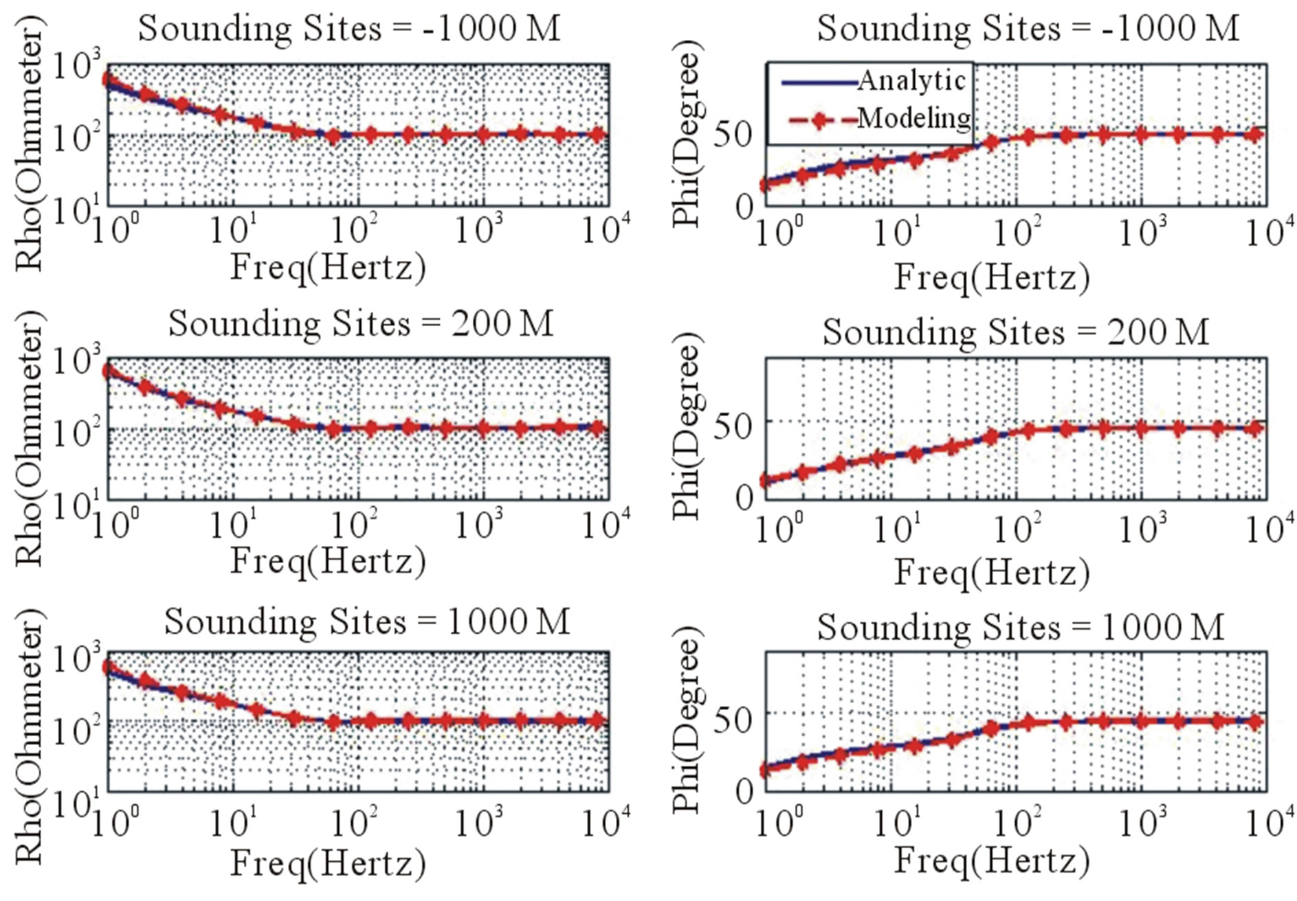
Figure 4. The comparison of apparent resistivity (left) and phase of impedance(right) of analytical calculation sandnumerical modeling for CSAMT sounding point –1000 m (top), 200 m (middle) and 1000 m (bottom) for homogeneous earth model with xy configuration.
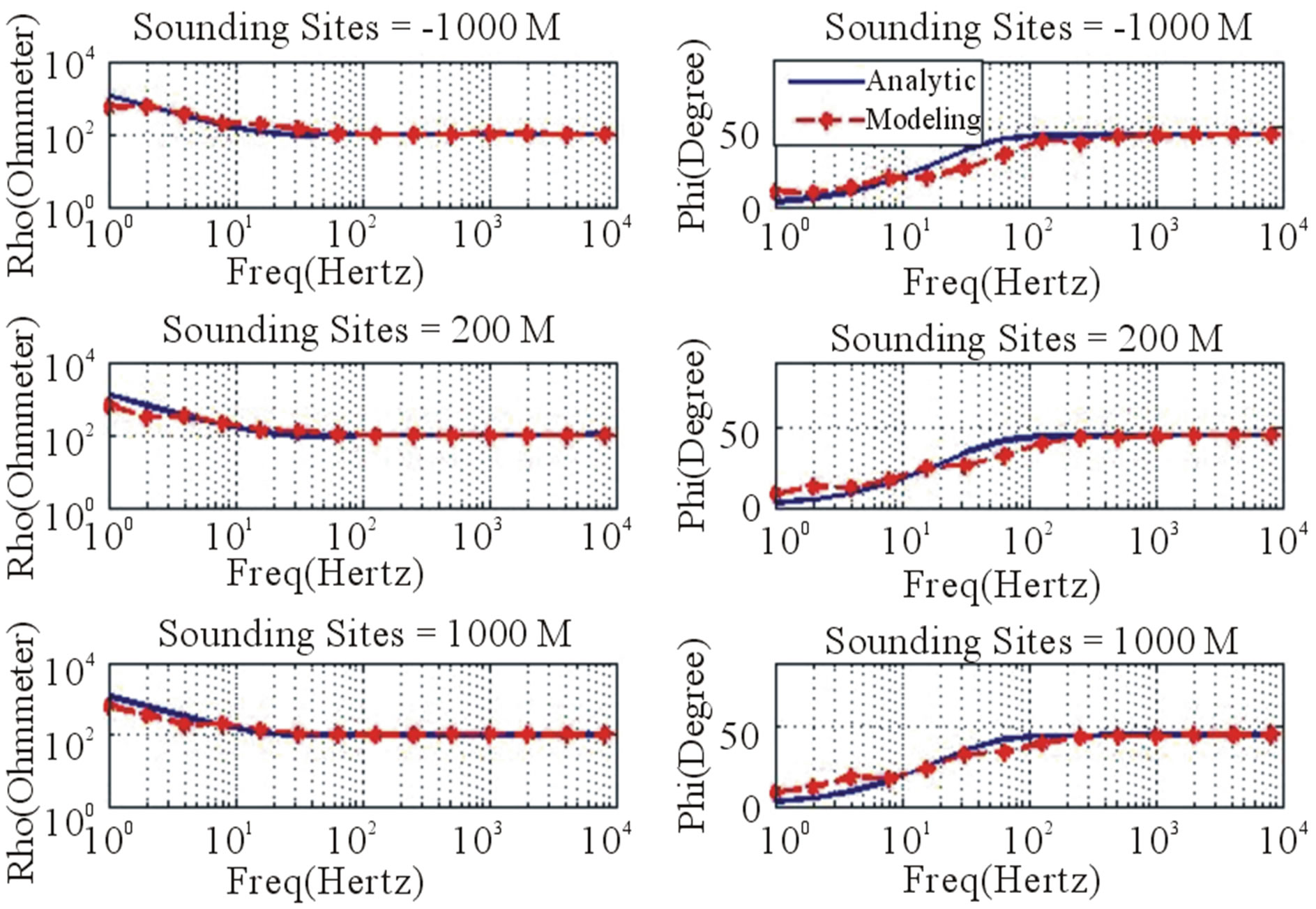
Figure 5. The comparison of apparent resistivity (left) and phase of impedance (right) of analytic calculation and numerical modeling of CSAMT-yx configuration for homogeneous earth model.
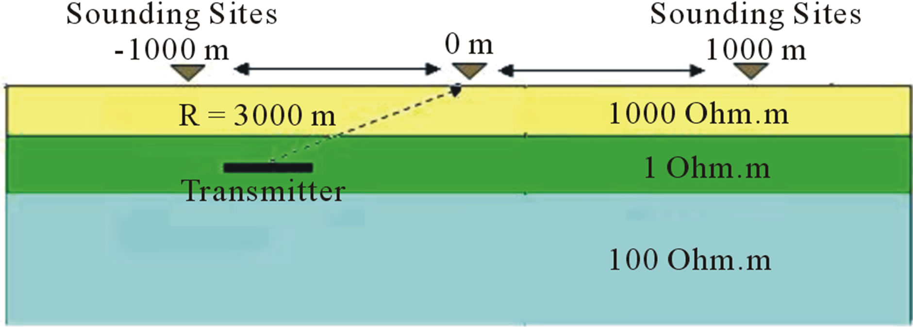
Figure 6. Three layers earth model.
range of tolerances. The highest error rate is about 6% for the apparent resistivity of layered earth with yx configuration. The validation indicates that the modeling scheme are reasonably valid to model 1D responses, and the modeling scheme can be used as the primary field in the modeling of the secondary field for the 2D cases.
The modeling of 2D cases consists of two models: 1) the vertical contact model, and 2) the conductive prism in
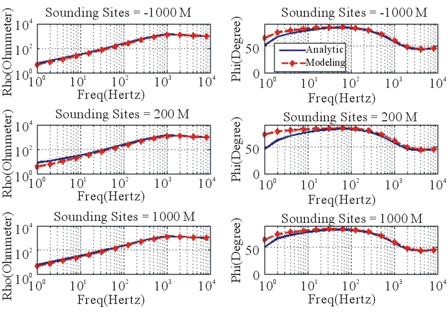
Figure 7. The comparison of apparent resistivity (left) and phase of impedance (right) of analytic calculation and numerical modeling of CSAMT-xy configuration for layered earth model.
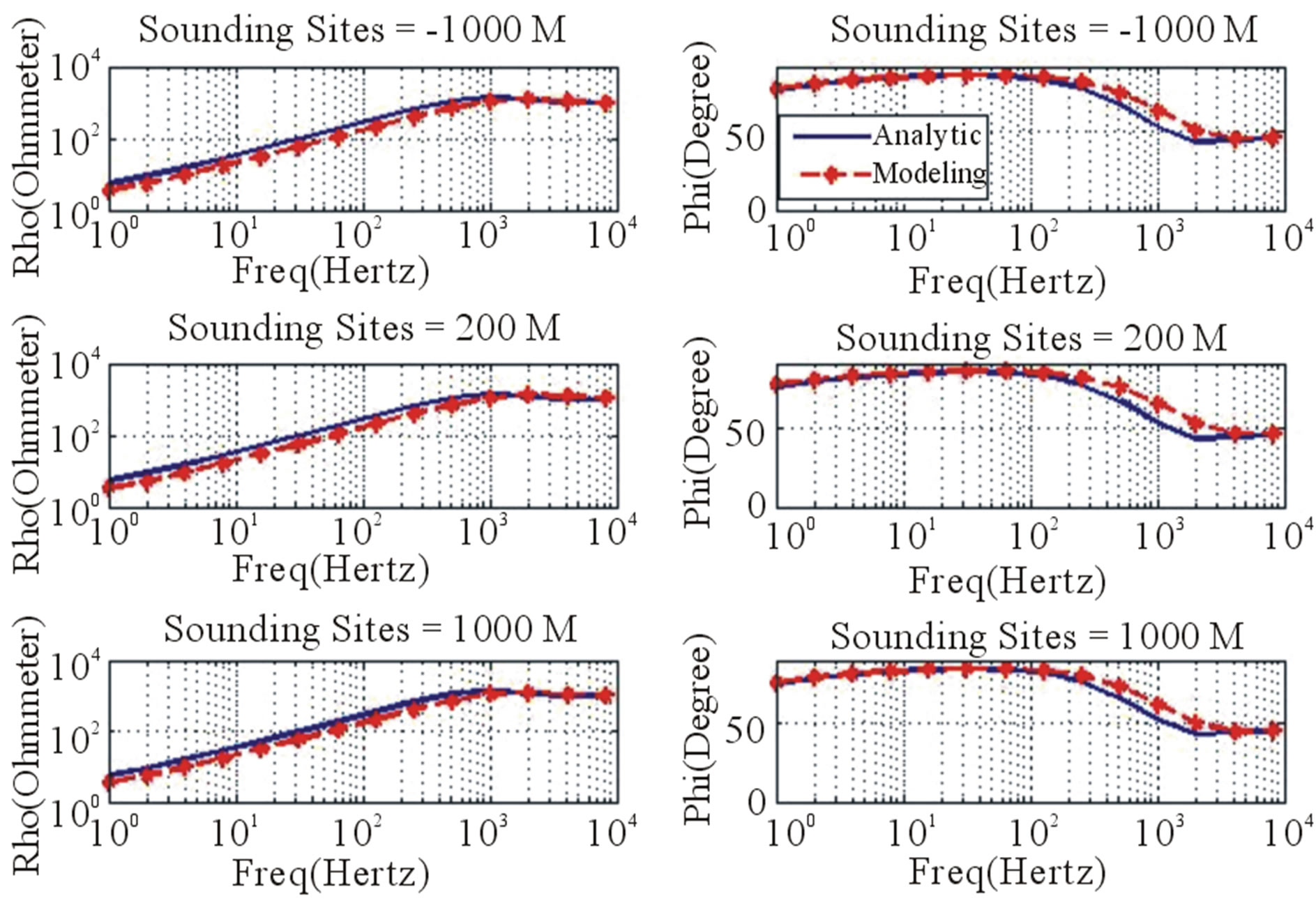
Figure 8. The comparison of apparent resistivity (left) and phase of impedance (right) of analytic calculation and numerical modeling of CSAMT-yx configuration for homogeneous earth model
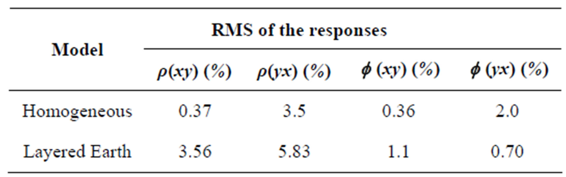
Table 1. Relative RM Serror of apparent resistivity (ρ) and phase of impedance ( ) of the modeling results compared to analytical solutions.
layered earth model. The responses generated by modeling are then compared to MT responses, using the MT TE code developed by Srigutomo and Sutarno [26]. Vertical contact model consists of two blocks with resistivity of 100 and 1 Ohm-meters (Figures 9). The last model consists of two layer earth model with conductive prism lying in the second layer, represent the anomalous body inside layered earth. Host rock resistivity is 100 meters, with 1 Ohm-meters conductive prism located 300 meters below the surface, precisely lying under the top of a 1000 Ohm-meters cap rock (Figure 10).
According to Figure 9, the geological strike is assumed perpendicular to the transmitter orientation, i.e. paralel to the y axis. Thus, the Ex and Hx components are perpendicular to strike direction, while the Ey and Hy are parallel to the strike. The modeling is conducted in xy configuration in which electric field is perpendicular to the strike, and yx configuration in which the electric field is parallel to the strike. For the yx configuration, the magnetic field parallel to transmitter Hx is set as the primary field, and the electric field perpendicular to transmitter Ey is calculated using the curl operation of the total magnetic field as in Equation (13). In the xy configuration, the perpendicular-to-transmitter magnetic field Hy is measured by the rotation of the total electric field parallel to the transmitter Ex as shown in Equation (10). The apparent resistivity and phase of impedance are calculated using Equations (11) and (14).
Figures 11 and 12 show the profiling responses generated by vertical contact model, for both CSAMT in xy and yx configurations and TE-MT. The frequencies for profiling are 8 Hz, 32 Hz, 128 Hz, 512 Hz, 2048 Hz and 8192 Hz. These frequencies were chosen to describe the rate of change per decade of frequency responses. From Figure 11, the apparent resistivity from both CSAMT-yx and MT-TE shows relatively similar results, while the CSAMT-xy shows relative different behavior. The CSAMT-xy configuration can be assumed as TM modes since the electric field is perpendicular to the strike direction, while the yx configuration can be assumed as TE modes. This explains the behavior of the responses: the yx response shows similar behavior with MT-TE, and
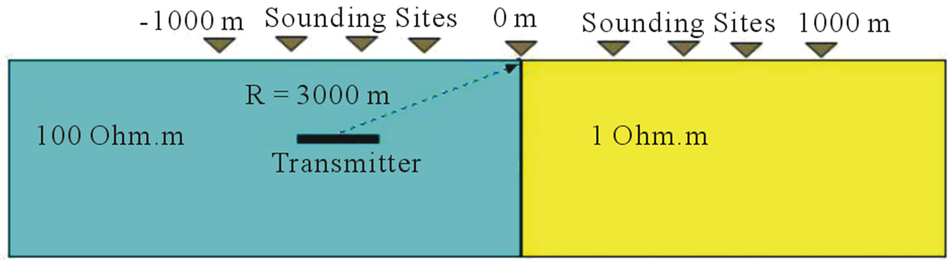
Figure 9. The vertical contact model.
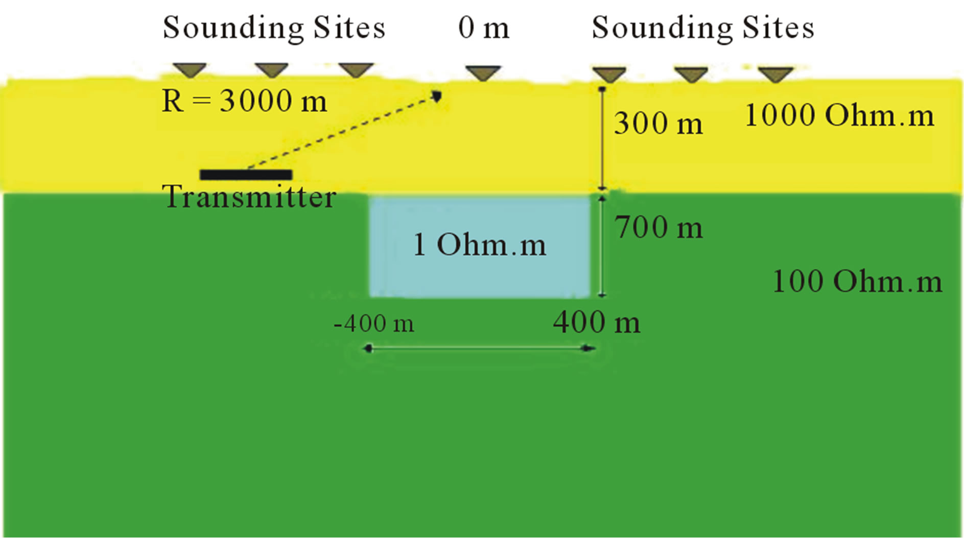
Figure 10. The conductive prism model.
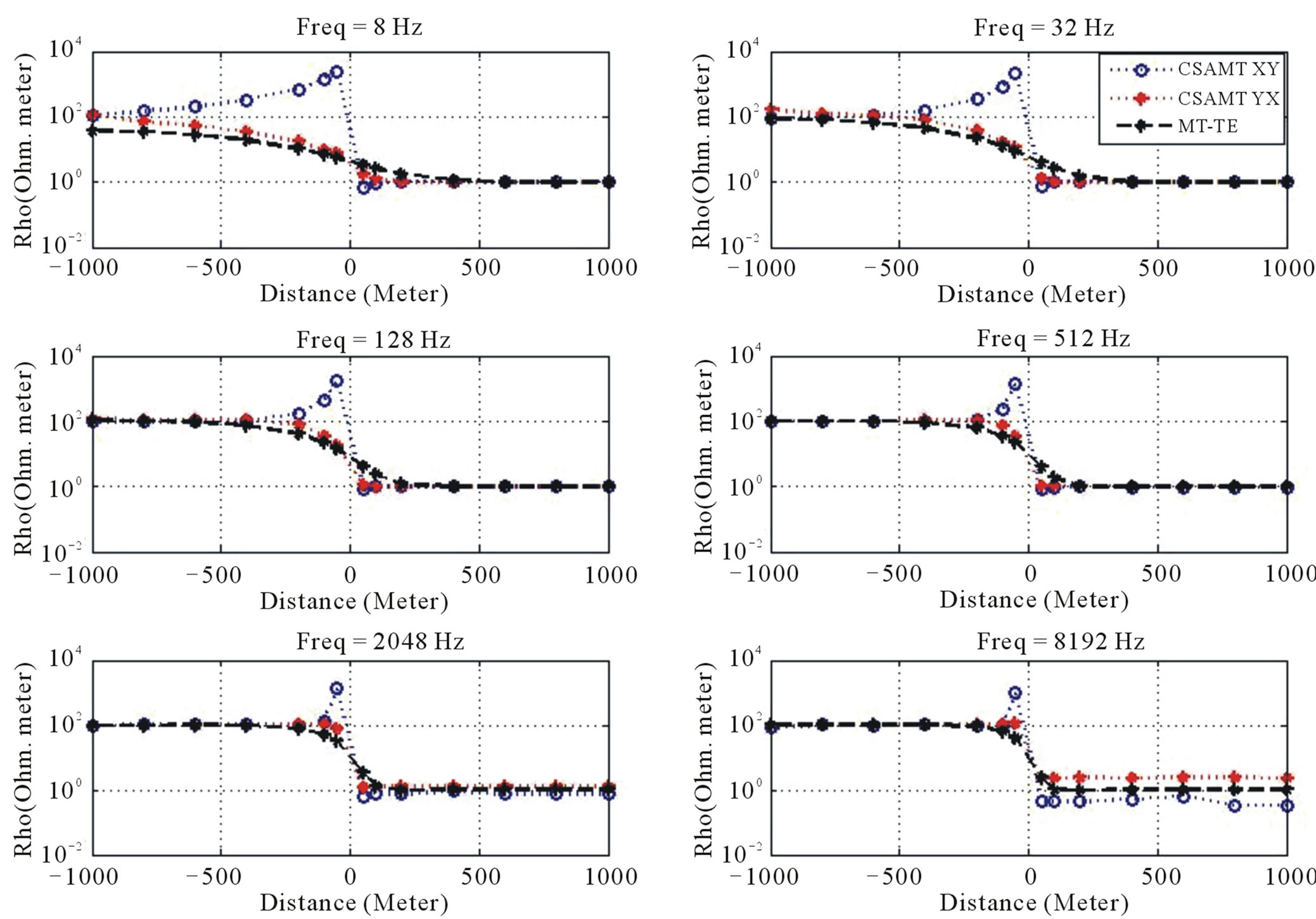
Figure 11. The vertical contact profiling of CSAMT apparent resistivities of xy and yx configurations, compared to MT-TE responses.
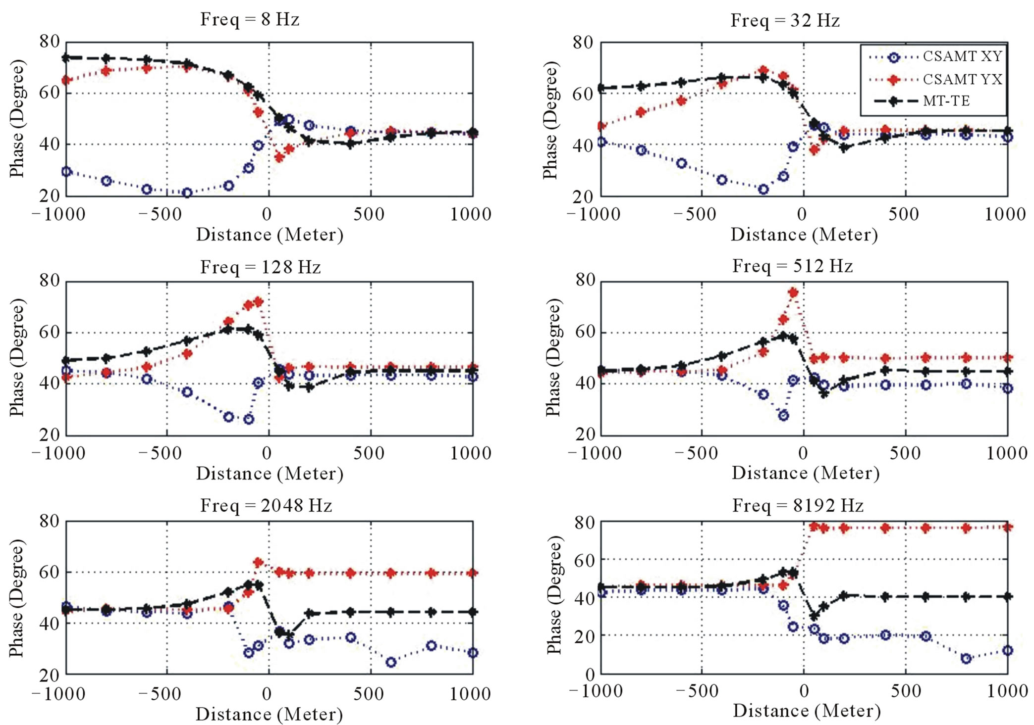
Figure 12. The vertical contact profiling of CSAMT phase of impedanceof xy and yx configurations, compared to MT-TE responses.
the xy configuration shows the behavior of TM polarization, which is described by discontinuous responses around the vertical contact. The phase of impedance generated by CSAMT, as shown in Figure 12, are more sensitive to the presence of vertical contact than MT. At low frequency, such as 8 Hz and 32 Hz, the xy configuration shows similar phase response to TE-MT, with relatively unsmooth change around the vertical contact. The abrupt changes around vertical contact are clearly shown in frequencies above 32 Hz. The phase of impedance response suggests that CSAMT responses are more sensitive to the presence of vertical contact than MT.
Figure 13 shows the pseudosection of CSAMT responses for both xy and yx configuration. The apparent resistivities for both configurations are clearly indicating the resistivity contrast due to vertical contact. The apparent resistivity of yx configuration is gradually changes, while the xy configuration shows relatively abrupt changes close to the vertical contact. The phase of impedance of xy configuration is scattered in high frequencies, while the yx configuration clearly shows the vertical contact in whole frequencies. Both apparent resistivities and phase of impedances pseudosection confirms the presence of vertical contact.
The direction of the electric field Ex in the xy configuration is perpendicular to the strike, which causes the discontinuity of electric field in vertical contact, and produces the surface current at the vertical boundary. The contrast apparent resistivity between the blocks is contributed by the current, and produces the sharp responses of xy configuration near the vertical contact area. The surface current is not obtained in the yx configuration, since the electric field perpendicular to the transmitter Ey has the same direction with the direction of lateral inhomogeneity, and it causes Ey field to be continuous across the boundary. Thus the existence of the contact area is smoothly described, following the smooth changes of electric field across the vertical contact.
The next model described is the case of conductive prisms lying on layered earth (see Figure 10). The responses of the model are shown in Figures 14-16.
The 1 Ohm meter conductive prism is buried 300 meters below the surface, at the top of 100 Ohm meter host rock. As in previous model, the responses are calculated by both xy and yx CSAMT configurations and compared to MT responses in six selected frequencies. The profil-
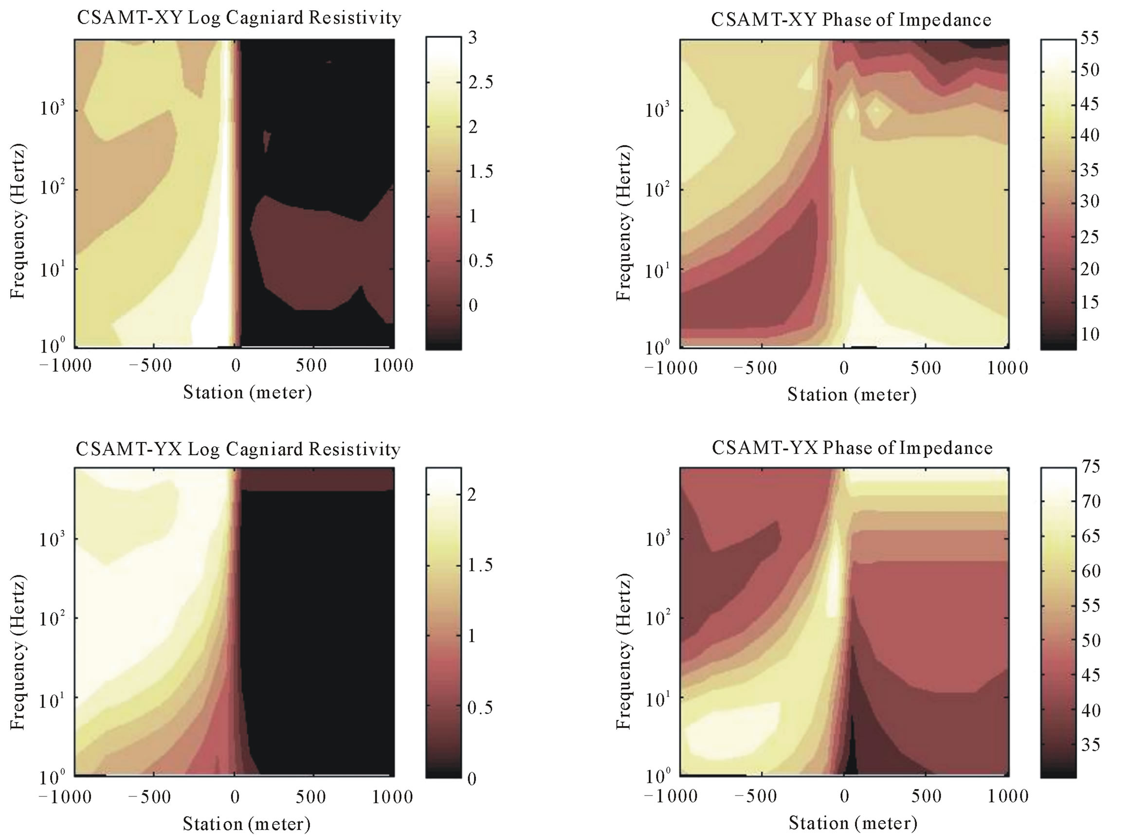
Figure 13. Pseudosection’s contour of CSAMT responses of vertical contact model for both xy and yx configurations.
ing of apparent resistivity on Figure 14 shows that xy configuration is more sensitive than yx configuration and MT. At the low frequency, such as 8 Hz and 32 Hz, the presence of conductive body is shown by undulate apparent resistivity responses. The CSAMT-xy resistivity response is more sensitive than yx, while the yx response still more sensitive than MT response. The phase of impedance responses in Figure 15 confirmed the sensitivity of xy response.
Pseudo section contour in Figure16 confirms the high sensitivity of xy configuration than yx configuration. The sensitivity of apparent resistivity contours in the xy configuration is characterized by the contour lines which described the presence of anomalous conductivity at locations around the anomalous objects, while the lines are tend to convex in yx configuration. In the pseudosection contour of phase of impedance, the xy mode contours clearly describe the location of anomalous objects, shown by the accumulation of phase’s low values at low frequencies. The yx phase of impedance also shows the accumulation of high value at high frequencies; describing the position of anomalous bodies. As described by the previous models, the pseudosection contour of CSAMT responses clearly indicates that sensitivity of xy responses is better than yx configuration. However, both configuration needs to be taken to get the complete picture of earth’s response.
In general, the modeling has successfully calculated the responses generated by CSAMT, and gives a better result than MT since the responses are more sensitive to detect the 2D anomalies. However, some aspects of this modeling need to be improved, e.g. the computational time and the numerical accuracy. The modeling is run using PC computer with 1 GB of memory and dual core processor 1.8 GHz, and using Conjugate Gradient Method (CGM) technique as the matrix solver. It takes about 10,000 seconds to get a response from one 2D model with 14 frequencies from 1 Hz to 8192 Hz. The development to improve the modeling performance consist of the use of sparse matrix solver to reduce the computational costs, and the use of high order elements such as quadratic and cubic elements, or using the edge elements [21] to give more accurate results.
5. Conclusion
The modeling developed in this study has successfully calculated the 2D CSAMT responses, confirmed by
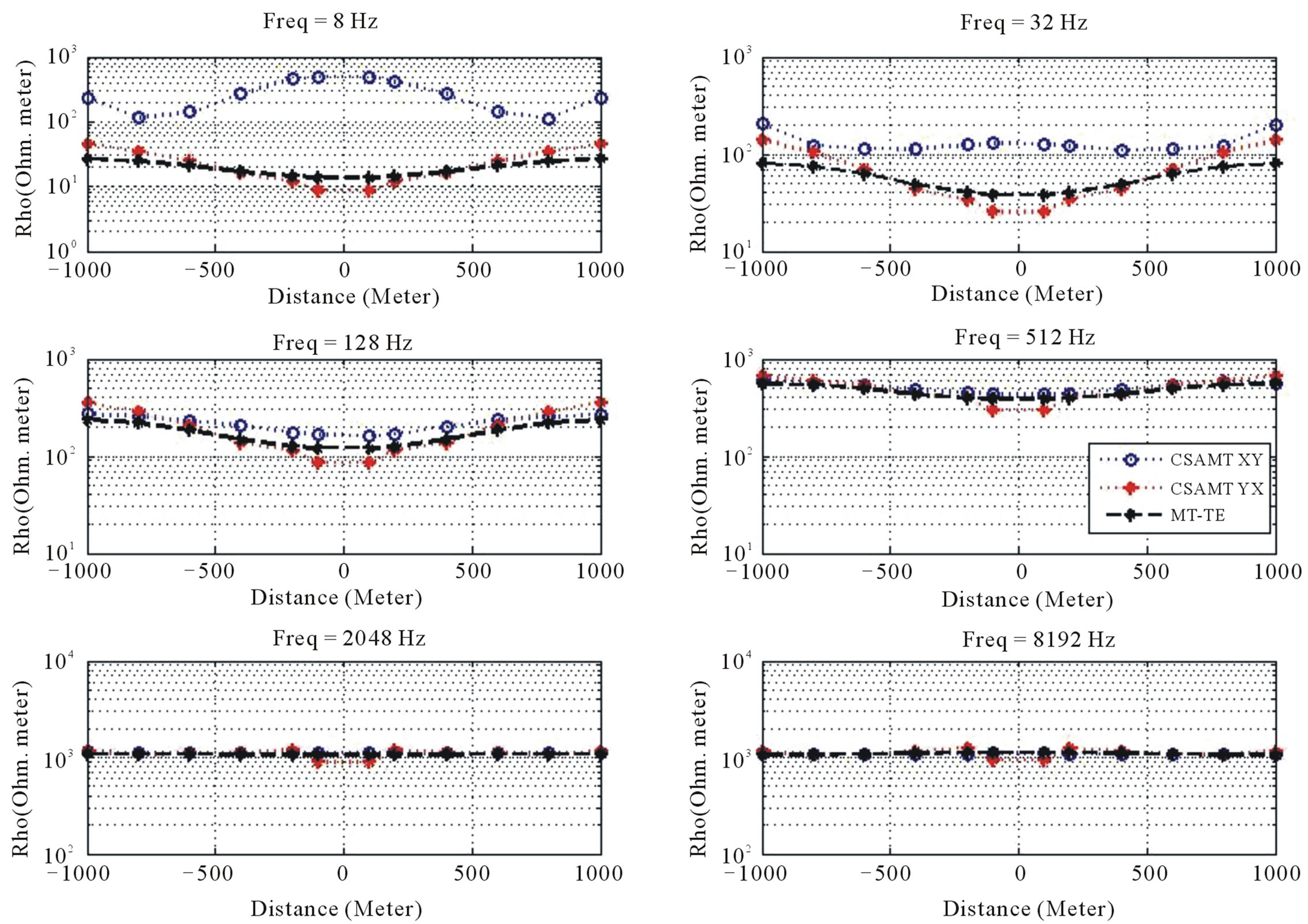
Figure 14. The profiling of conductive prism model of CSAMT apparent resistivities of xy and yx configurations, compared to MT-TE responses.
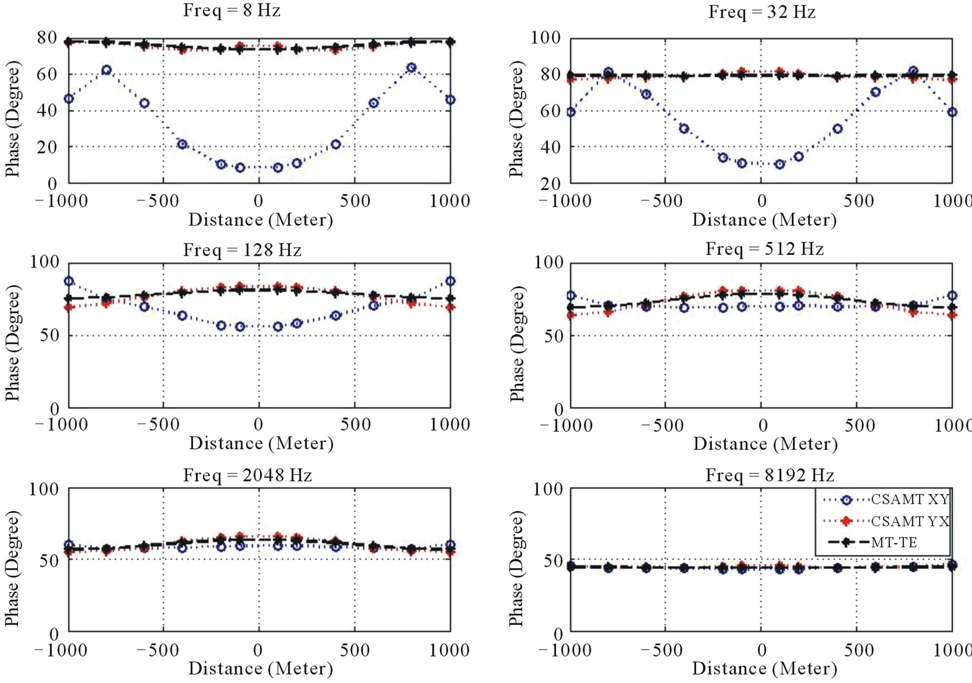
Figure 15. The profiling of conductive prism model of CSAMT apparent resistivities of xy and yx configurations, compared to MT-TE responses.
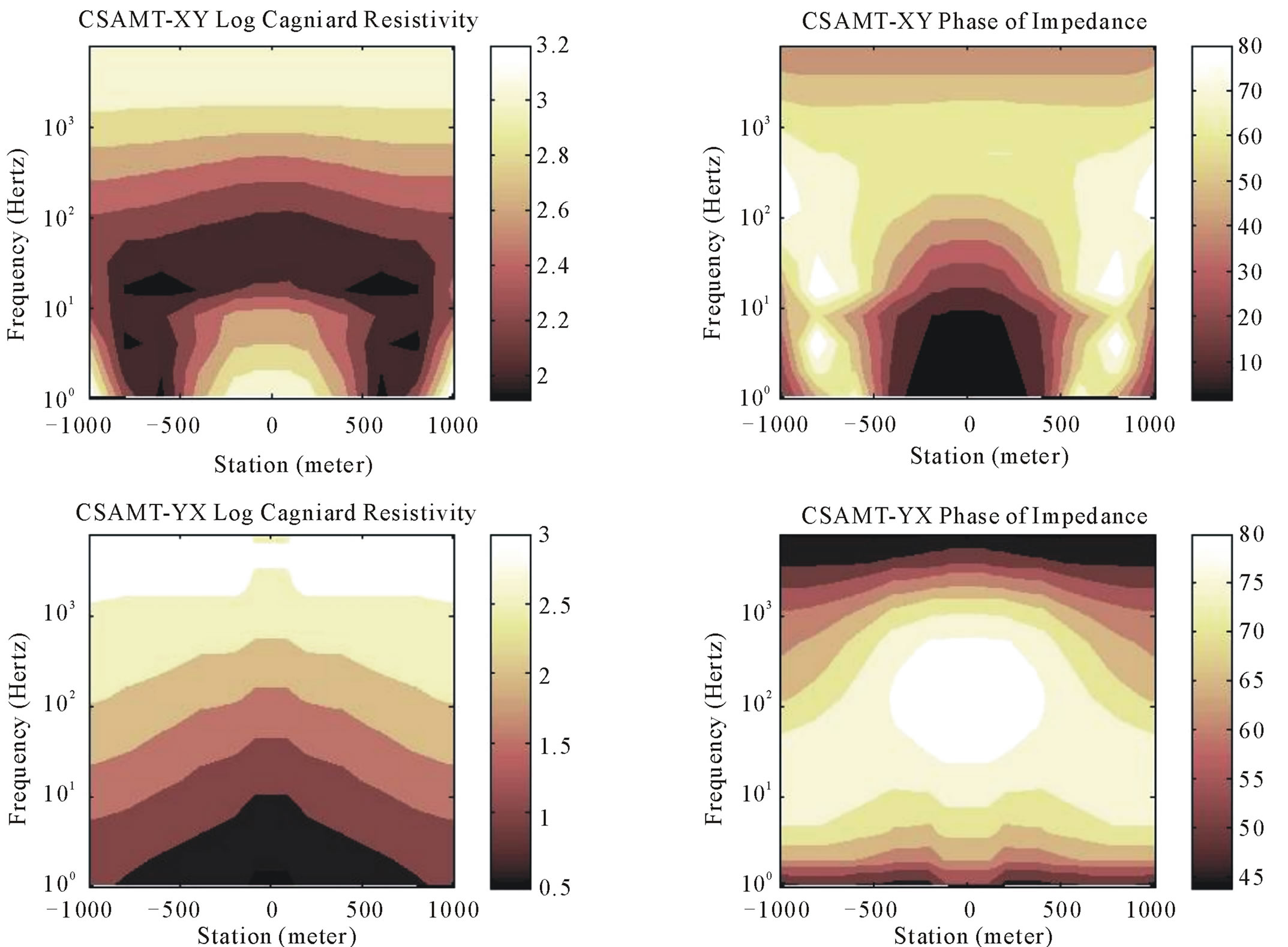
Figure 16. Pseudosection’s contour of CSAMT responses of conductive prism model for both xy and yx configurations.
validation with the 1D analytical results, which shows good compatibility between analytical and numerical results. The 2D modeling for vertical contact and conductive prism models confirms the superiority of CSAMT than MT in order to locate the anomalous bodies. The 2D modeling results also confirm the superiority of the configuration with electric field perpendicular to the strike direction than the electric field parallel to strike direction. Further developments are suggested to increase the accuracy of the results and reduce computational time.
6. Acknowledgements
We would like to express our gratitude to FMIPA ITB and LPPM-ITB for their support in this research. This research was funded by Riset ITB No. 248/K01.07/ PL/2009.
REFERENCES
- M. A. Goldstein and D. W. Strangway, “Audio-Frequency Magnetotellurics with a Grounded Electric Dipole Source,” Geophysics, Vol. 40, No. 4, 1975, pp. 669-683.
- S. K. Sandberg and G. W. Hohmann, “Controlled Source Audio Magnetotelluricsin Geothermal Exploration,” Geophysics, Vol. 59, 1982, pp. 100-116.
- P. E. Wannamaker, “Tensor CSAMT Survey over the Sulphur Springs Thermal Area, Valles Caldera, New Mexica, USA, Part I: Implications for Structure of the Western Caldera,” Geophysics, Vol. 62, No. 2, 1997, pp. 451- 465.
- P. E. Wannamaker, “Tensor CSAMT Survey over the Sulphur Springs Thermal Area, Valles Caldera, New Mexica, USA, Part II: Implications for CSAMT Methodology,” Geophysics, Vol. 62, No. 2, 1997, pp. 466-476.
- L. J. Hughes and N. R. Carlson, “Structure Mapping at Trap Spring Oilfield, Nevada Using Controlled-Source Magnetotellurics,” First Break, Vol. 5, No. 11, 1987, pp. 403-418.
- A. G. Ostrander, N. R. Carlson and K. L. Zonge, “Further Evidence of Electrical Anomalies over Hydrocarbon Accumulations Using CSAMT,” 53rd Annual SEG Meeting, Dallas, Expanded Abstracts, 1983, pp. 60-63.
- L. C. Bartel and R. D. Jacobson, “Results of a Controlled Source Audio Frequency Magnetotelluric Survey at the Puhimau Thermal Area,” Geophysics, Vol. 52, 1987, pp. 665-677.
- Y. Sasaki, Y. Yoshihiro and K. Matsuo, “Resistivity Imaging of Controlled-Source Audio Frequency Magnetotelluric Data,” Geophysics, Vol. 57, No. 7, 1992, pp. 952-955.
- M. Yamashita, P. G. Hallof and W. H. Pelton, “CSAMT Case Historis with a Multichannel CSAMT System and near Field Data Correction,” 55th SEG Annual Convention, 1985, pp. 276-278.
- A. A. Kaufmann and G. V. Keller, “Frequency and Transient Sounding,” Elsevier, Amsterdam, 1983.
- S. H. Ward and G. W. dan Hohmann, “Electromagnetic Theory for Geophysical Applications,” In: M. N. Nabighian, Ed., Electromagnetic Methods, Theory and Practice, Society of Exploration Geophysicist, Vol. 1, 1988, pp. 131-311.
- N. P. Singh and T. Mogi, “EMDPLER: A F77 Program for Modeling the EM Response of Dipolar Sources over the Non-Magnetic Layer Earth Model,” Computer and Geosciences, Vol. 36, No. 4, 2010, pp. 430-440. doi:10.1016/j.cageo.2009.08.009
- C. H. Stoyer and R. J. Greenfield, “Numerical Solutions of the Response of a Two Dimensional Earth to an Oscillating Magnetic Dipole Source,” Geophysics, Vol. 41, No. 3, 1976, pp. 519-530.
- M. J. Unsworth, B. J. Travis and A. D. Chave, “Electromagnetic Induction by a Finite Electric Dipole Source over a 2D Earth,” Geophysics, Vol. 58, No. 2, pp. 198- 214.
- Y. Mitsuhata, “2D Electromagnetic Modeling by FiniteElement Method with a Dipole Source and Topography,” Geophysics, Vol. 65, No. 2, 2000, pp. 465-475.
- Y. Li and K. Key, “2D Marine Controlled-Source Electromagnetic Modeling: Part 1—An Adaptive Finite-Element Algorithm,” Geophysics, Vol. 72, No. 2, 2007, pp. 51-62.
- R. Streich, “3D Finite Difference Frequency Modeling of Controlled Source Electromagnetic Data: Direct Solution and Optimization for High Accuracy,” Geophysics, Vol. 74, No. 5, 2009, pp. 95-105.
- K. H. Lee and H. F. Morrison, “A Numerical Solution for Electromagnetic Scattering by a Two Dimensional Inhomogenity,” Geophysics, Vol. 50, No. 3, 1985, pp. 1163- 1165.
- N. B. Boschetto and G. W. Hohmann, “Controlled Source Audiofrequency Magnetotelluric Responses of Three Dimensional Bodies,” Geophysics, Vol. 56, No. 2, 1991, pp. 255-265.
- G. A. Newman, G. W. Hohmann and W. L. Anderson, “Trans- ient Electromagnetic Response of a Three-Dimensional Body in a Layered Earth,” Geophysics, Vol. 51, No. 8, 1986, pp. 1608-1627.
- J. M. Jin, “The Elemen Hingga Method in Electromagnetic,” John Wiley & Sons, Singapore City, 1993.
- W. L. Anderson, “Numerical Integration of Related Hankel Transform of Order 0 and 1 by Adaptive Digital Filtering,” Geophysics, Vol. 44, No. 7, 1979, pp. 1287-1305.
- W. L. Anderson, “A Hybrid Fast Hankel Transforms Algorithm for Electromagnetic Modeling,” Geophysics, Vol. 54, No. 2, 1989, pp. 263-266.
- W. G. Hohmann, “Numerical Modeling for Electromagnetic Methods of Geophysics,” In: M. N. Nabighian, Ed., Electromagnetic Methods Theory and Practice, Society of Exploration Geophysicist, Vol. 1, pp. 131-311.
- K. L. Zonge and L. J. Hughes, “Controlled Source Audio-Frequency Magnetotellurics,” In: M. N. Nabighian, Ed., Electromagnetic Methods in Applied Geophysics, Society of Exploration Geophysicists, Tulsa, Vol. 2, 1991, pp. 713-809.
- W. Srigutomo and D. Sutarno, “Pemodelan Elemen Hingga Respon Elektromagnetik 2D Untuk Sumber Gelombang Bidang,” Kontribusi Fisika Indonesia, Vol. 9. No. 2, 1998, pp. 55-65.