Journal of Electromagnetic Analysis and Applications
Vol. 3 No. 8 (2011) , Article ID: 6635 , 8 pages DOI:10.4236/jemaa.2011.38051
Crosstalk Prediction for Three Conductors Nonuniform Transmission Lines: Theoretical Approach & Numerical Simulation
![]()
Research Unit Systems of Telecommunications (6’Tel), SUP’COM, University of the Carthage, Ariana, Tunisia.
Email: mnaouer.kachout@supcom.rnu.tn
Received June 15th, 2011; revised July 14th, 2011; accepted July 22nd, 2011.
Keywords: Nonuniform Transmission Lines, Near-End Crosstalk, Far-End Crosstalk
ABSTRACT
In this paper the crosstalk between nonuniform transmission lines is examined. Firstly, methods for prediction of crosstalk between microstrip transmission lines are reviewed. Classical coupled transmission line theory is used for uniform lines and cannot be used for nonuniform transmission lines. Secondly, equations are derived which can be solved to obtain formulas for the near-end and far-end crosstalk for nonuniform transmission lines. Finally, an example is worked which illustrates the crosstalk between three conductor nonuniform transmission lines. Obtained theoretical results were compared with simulations data. Comparison results shown that theoretical and simulation results are approximately the same.
1. Introduction
Modern trends in circuit designs such as operating at higher frequencies [1], lowering threshold voltages, and shrinking device geometries have made accurate prediction of electromagnetic compatibility (EMC) an indispensable component in the design cycle [2,3]. Susceptibility to electromagnetic interference (EMI) can severely degrade the signal integrity of the system [4,5]. One of the main sources for the EMI is the coupling between incident EM field and the electrical interconnects, which serve as antennas at high frequencies [6].
The problem of characterizing the coupling between interconnects are typically related to multiconductor transmission lines (MTLs) and coupled non-uniform transmission lines (NTLs). Coupled NTLs are widely used in RF and microwave circuits [7,8]. Coupled NTLs are encountered in many interconnects and packaging structures. Also, some of NTLs structures such as the tapered ones, have found important applications in narrowband microwave circuits.
The differential equations describing coupled NTLs have non-constant matrices, so except for a few special cases no analytical solution exists for them. Some methods such as decoupling [9,10], finite difference [11]Taylor’s series expansion [12], Fourier series expansion [13], the equivalent sources method [14] and the method of moments [15] have been introduced to analyze coupled NTLs. In some of these methods such as finite difference and Taylor’s series expansion, it is necessary to use an optimization process to satisfy terminal conditions. This is due to the nature of terminal conditions in coupled NTLs, which are two-point type. In the other word, the analysis of NTLs is a Boundary Value Problem (BVP) naturally.
In this paper, we propose an approach to analyze coupled NTLs. The approach presented in this regard is based on the concept of cascading many short sections, which relies on using the analytical closed-form exponential matrix solution, available for MTLs only. In contrast to the special case of a uniform MTLs, and NTLs is characterized by per-unit-length parameter matrices that are not constant, but rather vary with the spatial dimension in the telegraphers equations. This fact makes handling the line more challenging, since a closed-form solution cannot be obtained analytically except in special situations. In this work we develop rigorous equations to predict crosstalk between coupled NTLs.
This paper is organized as follows. Section 2 presents a brief background on formulating MTLs. In Section 3 we derive the literal or symbolic solution of the coupled NTLs equations for three conductor nonuniform transmission lines. Section 4 presents numerical validations by comparing theoretical with simulation results and discuss some concluding remarks
2. State of the Art
The literature on crosstalk between transmission lines dates back at least to the 1930s, and textbooks have been written on MTLs. Strictly speaking, classical transmission line theory applies only to perfectly conducting lines in a homogeneous medium so that the transmission line modes are transverse electromagnetic (TEM). The basic idea to study the coupling between NTLs is to cascade many short sections (by dividing the non-uniform line to “n” small equal uniform lines). In this section, we present the state of the art of coupling between three conductor transmission lines. The goal of this section is to demonstrate that using the existing theory of MTLs we cannot calculate the coupling between NTLs.
2.1. Theoretical Study of Uniform MTLs
Microstrip lines do not support pure TEM modes, but at low frequencies they support quasi-TEM modes that approximately satisfy the transmission line equations.
A cross-sectional view of a pair of microstrip lines on a grounded substrate is shown in Figure 1. For simplicity, we assume that the two strips have equal width w, zero thickness, and perfectly conductivity. The ground plane is also assumed to be perfectly conducting. The lines are located on a dielectric slab (substrate) of thickness h and have a separation s. The substrate has relative permittivity εr and free-space permeability μ0. The region above the substrate is free space.
The multiconductor transmission line equations can be compactly written in matrix form, but for discussion we choose to write out the coupled differential equations. For the source-free case, the line currents, I1 and I2, and voltages, V1 and V2, satisfy:
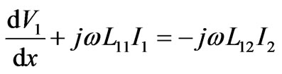 (1)
(1)
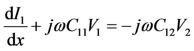 (2)
(2)
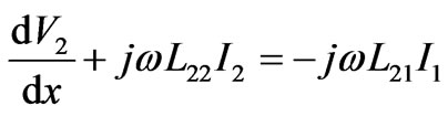 (3)
(3)
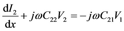 (4)
(4)
where x is the longitudinal coordinate and the exp(jωt)
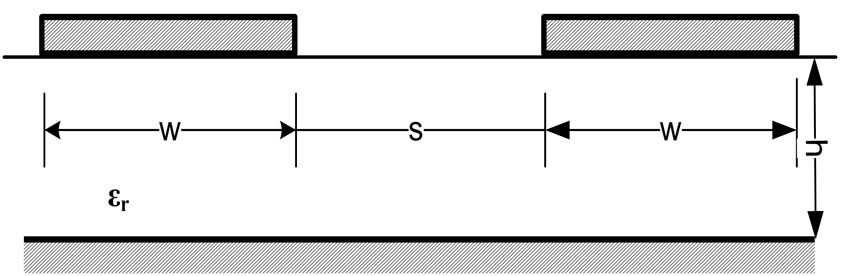
Figure 1. Cross-sectional geometry for a pair of identical microstrip transmission lines.
time dependence is suppressed. The Cij are the elements of the distributed capacitance matrix, and the Lij are the elements of the distributed inductance matrix.
Both the capacitance and inductance matrices are symmetric (C12 = C21 and L12 = L2l). Because of the microstrip symmetry, we also have C11 = C22 and L11 = L22.
For perfect conductors in a homogeneous dielectric, the capacitance and inductance matrices are frequency independent. When the dielectric region is inhomogeneous (as for insulated wires or microstrips), then the, capacitance and inductance matrices depend on frequency. However, they are approximately frequency independent over a large quasi-static frequency range.
The symmetric microstrip supports an even mode with V1 = V2 and an odd mode with V1 = –V2. The even and odd mode propagation constants are given by Equations (5) and (6).
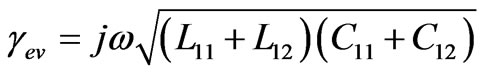 (5)
(5)
and
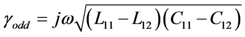 (6)
(6)
The even and odd mode characteristic impedances, Zev and Zodd, are:
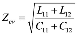 (7)
(7)
and
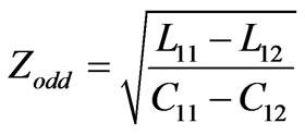 (8)
(8)
Equations (5) and (7) are deceptively simple because computation of the Lij and Cij elements generally requires some numerical method, such as the method of moments.
For large spacing (s/w  l), the coupling capacitance C12 and inductance L12 become small. In this case, the propagation constants in Equation (5) approach that of an isolated line γ0:
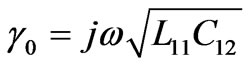 (9)
(9)
Also, the characteristic impedances in Equation (7) approach that of an isolated line Z0:
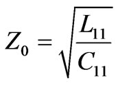 (10)
(10)
2.2. Crosstalk Predictions
To study crosstalk, we consider the geometry in Figure 2. The coupled microstrip lines are identical to those in Figure 1 except that they are of finite length l. Line 1 is fed with a voltage generator V = 0 at x = 0, and all four ports are terminated with an impedance Z0 We label the driven and terminated ends of line 1 as ports 1 and 2, and the near and far ends of line 2 as ports 3 and 4. The geometry in Figure 2 has been analyzed for both directional coupler applications and crosstalk predictions.
For crosstalk prediction, we can assume that the lines are loosely coupled (s is not too small compared to h and w). In this case, we can use the approximate solution of and equate near-end and far-end crosstalk to the S parameters as follows:
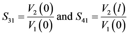 (11)
(11)
In terms of the microstrip parameters, S31 is approximately:
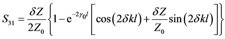 (12)
(12)
where
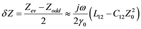 (13)
(13)
and
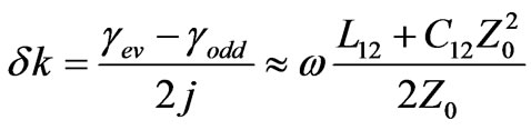 (14)
(14)
Similarly, S41 is approximately:
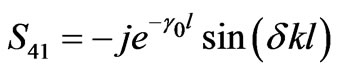 (15)
(15)
The transmission S parameter S21 is not needed for crosstalk prediction, but is approximately:
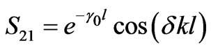 (16)
(16)
To first order in δz, the reflection coefficient S11 = 0. To first order in δz, the approximate S parameters satisfy conservation of power:
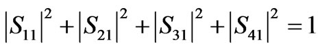 (17)
(17)
At sufficiently low frequencies (or for sufficiently short lines), we can assume that . In that case
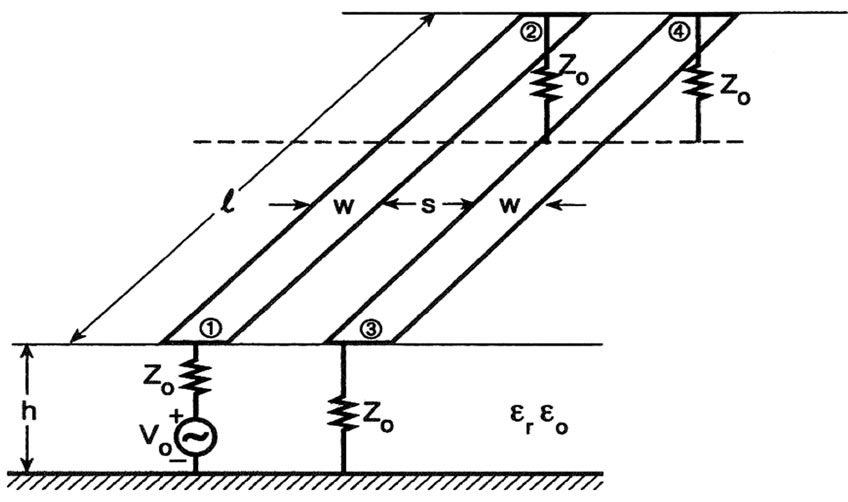
Figure 2. Two identical microstrip lines terminated in the characteristic impedance Z0 an isolated line. Line 1 is excited at port 1.
the scattering parameters of the previous section reduce to
 (18)
(18)
 (19)
(19)
and
 (20)
(20)
After rigorous theoretical study of existing solutions to calculate the coupling between uniform lines, we conclude that solutions detailed above do not take into account the non-uniformity of the lines. To do so, in the next section we develop theoretical solution to calculate the coupling between coupled NTLs. We must take into account the intrinsic characteristics of each physical part of the line
3. Coupled Nonuniform Transmission Lines
The purpose of this section is to derive the literal or symbolic solution of the coupled NTLs equations for three conductor nonuniform transmission lines and to incorporate the terminal impedance constraints into this solution to yield explicit equations for the crosstalk.
In order to understand the general behavior of the solution, it would be helpful to have a literal solution for the induced crosstalk voltages in terms of the symbols for the line length, terminal impedances, per-unit-length capacitances and inductances, the source voltage, etc. From such a result we could observe how changes in some or all of these parameters would affect the solution. This advantage is similar to a transfer function which is useful in the design and analysis of electric circuits and automatic control systems. In order to obtain this same insight from the numerical solution we would need to perform a large set of computations with these parameters being varied over their range of anticipated values.
Such transmission-line literal transfer functions for the prediction of crosstalk have been derived in the past for use in the frequency-domain analysis of microwave circuits or for time-domain analysis of crosstalk in digital circuits. However, all of these methods make one or more of the following assumptions about the line in order to simplify the derivation:
· The line is a three-conductor, with two signal conductors and a reference conductor.
· The line is symmetric, i.e., the two signal conductors are identical in cross-sectional shape and are separated from the reference conductor by identical distances
· The line is weakly coupled, i.e., the effect of the induced signals in the receiving circuit on the driven circuit is neglected (widely separated lines tend to satisfy this in an approximate fashion the wider the separation)· Both lines are matched at both ends (the line is terminated at all four ports in the line characteristic impedances).
· The line is lossless, i.e., the conductors are perfect conductors and the surrounding medium is lossless.
· The medium is homogeneous.
The obvious reason why these assumptions are used is to simplify the difficult manipulation of the symbols that are involved in the literal solution.
A nonuniform three-conductor transmission lines structure is sketched in Figure 3. The per-unit-length equivalent circuit is shown in Figure 4.
A voltage source VS(t), with internal resistance RS, is connected to a load RL via both a generator conductor and reference conductor. A receptor circuit shares the same reference conductor and connects two terminations RNE and RFE by a receptor conductor.
We subdivide this structure into “n” equal parts (Δ1, Δ2  Δn), each part have the same line length. In all these parts, conductors are assumed to be uniform. In this case, nonuniform lines can be considered as a coupled multiconductor transmission line.
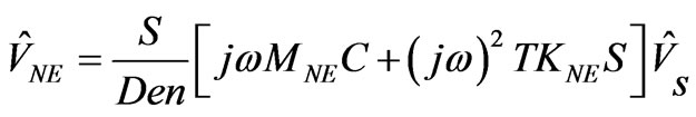
The near-end and far-end crosstalk voltages are obtained from the second entries in these solution vectors as .
.
The exact literal solution for the crosstalk voltages is:
 (21)
(21)
 (22)
(22)
 (23)
(23)
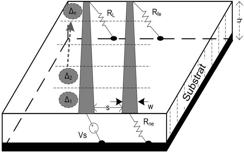
Figure 3. Coupled nonuniform transmission lines.
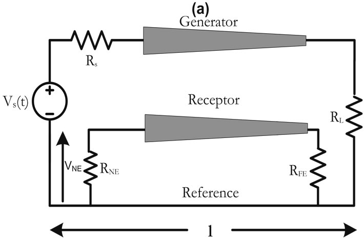
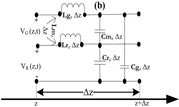
Figure 4. (a) Three-conductor transmission lines illustrating crosstalk; (b) per-unit length parameter.
The various quantities in these equations are:
 (24)
(24)
 (25)
(25)
where the inductlve-coupling coefficients are:
 (26)
(26)
 (27)
(27)
where lmi is the metual inductance for each part Δi of the line. And the capacitive-coupling coefficients are:
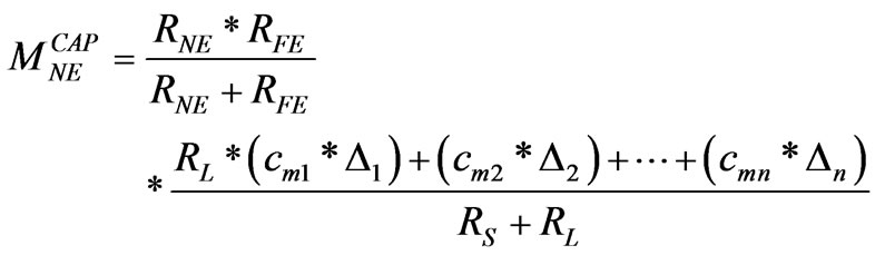 (28)
(28)
where Cmi is the metual capacitance for each part Δi of the line.
 (29)
(29)
The remaining quantities are defined in the following way. The coefficient KNE is defined by
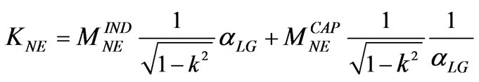 (30)
(30)
The coupling coefficient between the two circuits is defined by
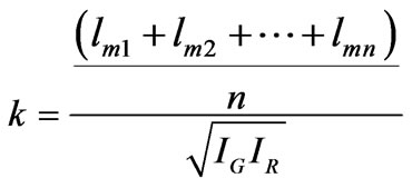 (31)
(31)
and the circuit characteristic impedances are defined by:
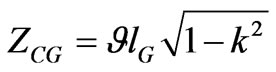 (32)
(32)
 (33)
(33)
The line one-way delay is denoted by:
 (34)
(34)
The relationships of the termination impedances to the characteristic impedances are important parameters. In order to highlight this dependency, the various ratios of termination impedance to characteristic impedance are defined by:
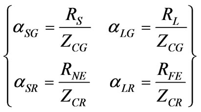 (35)
(35)
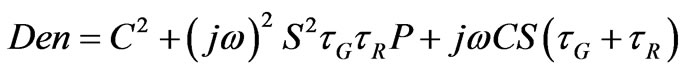
In terms of these ratios, the factor P in Den becomes:
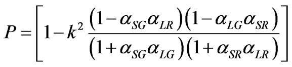 (36)
(36)
Observe that P = 1 if the line is weakly coupled,  , and/or the lines are matched at opposite ends,
  , or
, or . The circuit time constants are logically defined as:
 (37)
(37)
 (38)
(38)
Observe that a line time constant is equal to the line one-way delay if the lines are weakly coupled,  , and that line is matched at one end. In other words,
  if
if  and
and  or
or .
.
The above results are an exact literal solution for the problem. No assumptions about symmetry or matched loads are used. Therefore they cover a wider class of problems than have been considered in the past. Although they have been simplified by defining certain terms, they can be simplified further if we make the following assumptions. First let us assume that the line is electrically short at the frequency of interest, i.e., . In this case the terms C and S simplify to:
 (39)
(39)
 (40)
(40)
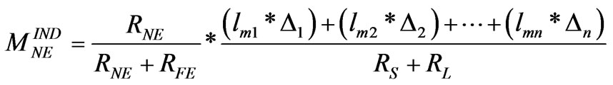
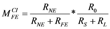
The near-end crosstalk can be viewed as a transfer function between the input VS(t) and the outputs VNE. This can be done by factoring out VS(t) and jω to give:
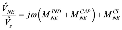 (41)
(41)
where
 (42)
(42)
Common impedance coupling in the near-end crosstalk can be evaluated using:
 (43)
(43)
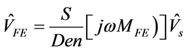
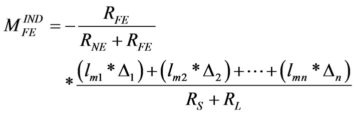
The far-end crosstalk is determined by:
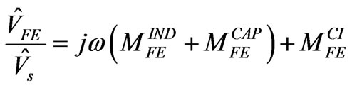 (44)
(44)
Common impedance coupling in the far-end crosstalk can be evaluated using:
 (45)
(45)
4. Simulation versus Theoretical Results
This section aims to validate theoretical proposed solution. We develop T-electric equivalent model for each part of the presented structure. Figure 5 shows the proposed
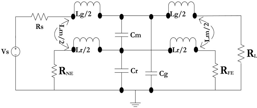
Figure 5. T-model.
T-model, where, Lm = lm*lw represents the mutual inductance between conductors, Lg = lg*lw is the self-inductance of generator conductor, Lr = lr*lw is the self-inductance of the receptor conductor. Where lw, lm, lg and lr denote the conductor length, the per-unit length mutual inductance between generator and receptor conductors, the per-unit length inductance of the generator conductor, and the per-unit length inductance of the receptor conductor, respectively. Cm = cm*lw is the mutual capacitance between conductors, Cr = cr*lw is the capacitance of receptor conductor, Cg = cg*lw is the capacitance of generator conductor. Where cm, cr and cg denote the per-unit length mutual capacitance between two conductors, the per-unit length capacitance of the receptor conductor, and the per-unit length capacitance of the generator conductor, respectively.
4.1. Nonuniform Conductors with Rectangular Cross-Section
In order to evaluate the crosstalk between nonuniform conductors, we deal first with various per-unit-length parameters. In principle, the method of moments is a common and widespread technique. In order to illustrate this method, let us reconsider the parallel-plate capacitor problem. We assume that the charge distribution over each plate is uniform, that is, does not vary over the plates. In reality, the charge distribution will peak at the edges. To model this, in Figure 6 we break each plate into small rectangular areas Δsi, and assume the charge over each subarea as being constant with an unknown level, αi. The total charge on each plate having been divided into N subareas is:
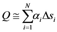 (46)
(46)
The heart of this method is to determine the total voltage of each subarea as the sum of the contributions from the charges on each subarea. Hence the total voltage of a subarea is the sum of the contributions from all the charges of all the subareas (including the subarea under consideration):
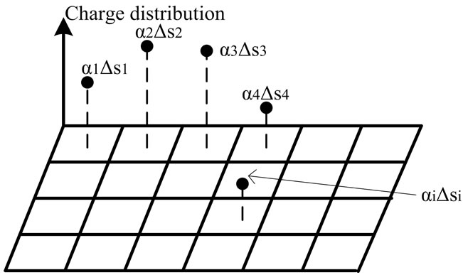
Figure 6. Approximating the charge distribution on the plates of parallel-plate capacitor.
 (47)
(47)
Each term Kji represents as basic subproblem relating the voltage of a subarea Vj to the charge amplitude on another subarea.
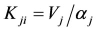 (48)
(48)
Because of symmetry (both plates are identical), we can assign the voltage of the top plate (with respect to infinity) as +V and the voltage of the bottom plate (with respect to infinity) as –V. The voltage between the two plates is then 2V, so that the capacitance is:
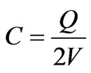 (49)
(49)
Grouping (70) for all subareas gives a matrix equation to be solved (which is the final result for all such MoM schemes):
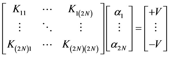 (50)
(50)
We have assigned all subareas on the top plate to have voltages of +V and all subareas on the bottom plate have voltages of –V. Once (50) is solved for all the αi charge distribution coefficients, the total charge on each plate can be determined from (46) and the total capacitance can be determined from (49).
In our case, we consider nonuniform transmission lines structure shown in Figure 3, where, h = 47 mils, and εr = 4,7 (glass epoxy). Conductors are assumed to be immersed in homogeneous medium.
The per-unit length capacitance parameter matrix is:
 (51)
(51)
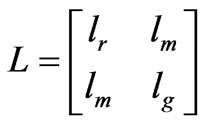
The per-unit length inductance parameter matrix is:
 (52)
(52)
In the configuration presented in Figure 3 we find that lr = lg and Cr = Cg.
For the above mentioned values and for “n = 5”, the per-unit length inductance and capacitance parameters for each part of the structure are presented in Table 1, where w is the line width and S is the separation distance between nonuniform conductors.
These parameters can now be used to simulate the mentioned electrical equivalent model; the model is implemented in Advanced design system (ADS) of Agilent. Figure 7 describes the near-end crosstalk variation versus frequency for nonuniform transmission lines.
Figure 7 shows a comparison between theoretical calculated near-end crosstalk results and simulation data. Results show that the coupling increases gradually versus frequency. For frequencies above 50 KHz, we can see that theoretical and simulation results are approximately the same.
4.2. Nonuniform Conductors with Circular Cylindrical Section
Conductors having cross sections that are circular cylindrical are referred to as wires. These are some of the few conductor types for which closed-form equations for the per-unit-length parameters can be obtained.
Three conductors, shown in Figure 8, have the radius varies from rw = 225 mils (Δn) to 125 mils (Δ1) and same length lw = 39370 mils separated by distance S varies from S = 100 mils (Δn) to 300 mils (Δ1). The configuration is assumed to be immersed in homogeneous medium (µ = µ0). The per-unit length inductance parameter matrix is:
 (53)
(53)
where
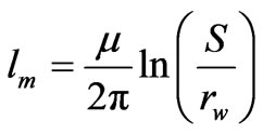 (54)
(54)
 (55)
(55)
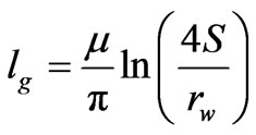 (56)
(56)
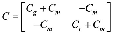
The per-unit length capacitance parameter matrix is:
 (57)
(57)
The relation between the per-unit length capacitance and inductance parameters matrix is given in Equation (58).
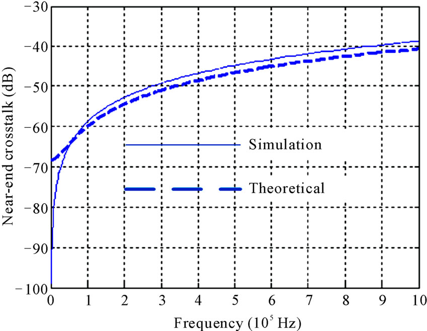
Figure 7. Comparison of theoretical and simulated near-end crosstalk.
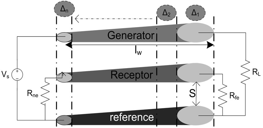
Figure 8. Nonuniform three-conductor transmission lines with circular cylindrical section.
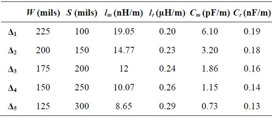
Table 1. Inductance and capacitance per-unit length parameters.
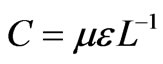 (58)
(58)
For the above mentioned values and for “n = 5”, the per-unit length inductance and capacitance parameters for each part of the structure are presented in Table 2, where rw is the conductor radius and S is the separation distance between nonuniform conductors.
These parameters can now be used to simulate the two explicated models.
Figure 9 shows a comparison between theoretical
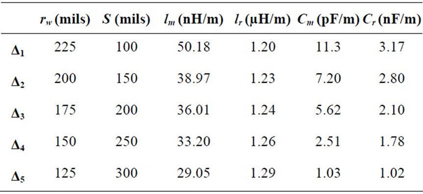
Table 2. Inductance and capacitance per-unit length parameters.
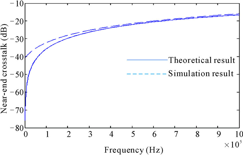
Figure 9. Comparison of theoretical and simulations results.
calculated near-end crosstalk results and simulation data using T models.
For frequencies above 100 KHz, we can see that theoretical and simulation results are approximately the same.
5. Conclusions
Rigorous equations have been developed to predict crosstalk between nonuniform transmission lines. Used conductors are assumed to be immersed in homogenous medium. Electric equivalent model has been presented for calculating the crosstalk between three-conductor nonuniform transmission lines. Rigorous equations are developed to calculate the per-unit length inductive and capacitive parameters. Comprehensive comparisons between the results which are obtained by using rigorous theoretical equations on one hand and those obtained by the created model on the other hand, have shown an excellent accuracy for higher frequencies. Theoretical solution for near-end and far-end crosstalk presented here are faster than the finite difference analysis.
REFERENCES
- K. Mnaouer, B. H. T. Jamel and C. Fathi, “Crosstalk Mitigation Enhanced by Reference Conductor Position,” 14th IEEE Workshop on Signal Propagation on Interconnects (SPI), Hildesheim, 9-12 May 2010. doi:10.1109/SPI.2010.5483549
- K. Mnaouer, B. H. T. Jamel and C. Fathi, “Shielded and Unshielded Three-Conductor Transmission Lines: Modeling and Crosstalk Performance,” 28th Progress in Electromagnetics Research Symposium (PIERS), Cambridge, 5-8 July 2010.
- K. Mnaouer, B. H. T. Jamel and C. Fathi, “Modeling of Microstrip and PCB Traces to Enhance Crosstalk Reduction,” IEEE R8 International Conference on Computational Technologies in Electrical and Electronics Engineering (SIBIRCON), Irkutsk, 11-15 July 2010.
- K. Mnaouer, B. H. T. Jamel and C. Fathi, “Development and Validation of an Electric Equivalent Models for Predicting Crosstalk Performance of Three-Conductor Transmission Lines,” 12th IEEE ICCS, Singapore City, 17-20 November 2010.
- K. Mnaouer, B. H. T. Jamel and C. Fathi, “Coupled Nonuniform Transmission Lines: Modeling and Crosstalk Performances,” 29th Progress in Electromagnetics Research Symposium (PIERS), Marrakesh, 20-23 March 2011.
- L. A. Hayden and V. K. Tripathi, “Nonuniform Coupled Microstrip Transversal Filters for Analog Signal Processing,” IEEE Transactions on Microwave Theory and Techniques, Vol. 39, No. 1, January 1991, pp. 47-53. doi:10.1109/22.64604
- T. Dhaene, L. Martens and D. D. Zutter, “Transient Simulation of Arbitrary Nonuniform Interconnection Structures Characterized by Scattering Parameters,” IEEE Transactions on Circuits and Systems, Vol. 39, No. 11, November 1992, pp. 928-937. doi:10.1109/81.199890
- M. Khalaj-Amirhosseini, “Analysis of Coupled Nonuniform Transmission Lines through Analysis of Uncoupled Ones,” International Symposium on Antennas and Propagation (ISAP’06), Singapore City, 1-4 November 2006.
- C. R. Paul, “Analysis of Multiconductor Transmission Lines,” John Wiley and Sons Inc., Hoboken, 1994.
- M. Khalaj-Amirhosseini, “Using Linear Sections Instead of Uniform Ones to Analyze the Coupled Nonuniform Transmission Lines,” International Journal of RF and Microwave Computer-Aided Engineering, Vol. 19, No. 1, 2009, pp. 75-79. doi:10.1002/mmce.20317
- M. Khalaj-Amirhosseini, “Analysis of Coupled or Single Non-uniform Transmission Lines Using Step-by-Step Numerical Integration,” Progress in Electromagnetics Research, PIER, Vol. 58, 2006, pp. 187-198. doi:10.2528/PIER05072803
- M. Khalaj-Amirhosseini, “Analysis of Coupled Non-uniform Transmission Lines Using Taylor’s Series Expansion,” IEEE Transactions on Electromagnetic Capability, Vol. 48, No. 3, 2006, pp. 594-600. doi:10.1109/TEMC.2006.879340
- M. Khalaj-Amirhossein, “Analysis of Periodic and Aperiodic Coupled Non-uniform Transmission Lines Using the Fourier Series Expansion,” Progress in Electromagnetics Research, PIER, Vol. 65, 2006, pp. 15-26. doi.:10.2528/PIER06072701
- M. Khalaj-Amirhosseini, “Analysis of Coupled or Single Non-uniform Transmission Lines Using the Equivalent Sources Method,” IEEE 2007 International Symposium on Microwave, Antenna, Propagation and EMC Technologies for Wireless Communications, (MAPE 2007), Hangzhou, 16-17 August 2007, pp. 1247-1250.
- M. Khalaj-Amirhosseini, “Analysis of Coupled or Single Nonuniform Transmission Lines Using the Method of Moments,” International Journal of RF and Microwave Computer-Aided Engineering, Vol. 18, No. 4, 2008, pp. 187-198. doi:10.1002/mmce.20295