Journal of Electromagnetic Analysis and Applications
Vol. 2 No. 7 (2010) , Article ID: 2333 , 7 pages DOI:10.4236/jemaa.2010.27055
Polynomial-Based Evaluation of the Impact of Aperture Phase Taper on the Gain of Rectangular Horns
![]()
Department of Physics, Aristotle University of Thessaloniki, Thessaloniki, Greece.
Email: kmpal@physics.auth.gr
Received March 28th, 2010; revised May 12th, 2010; accepted May 18th, 2010.
Keywords: Microwave Antennas, Rectangular Horn, Gain, Quadratic Phase Error, Linear Regression
ABSTRACT
The aperture phase taper due to quadratic phase errors in the principal planes of a rectangular horn imposes significant constraints on the on-axis far-field gain of the horn. The precise calculation of gain reduction involves Fresnel integrals; therefore, exact results are obtained only from numerical methods. However, in horns’ analysis and design, simple closed-form expressions are often required for the description of horn-gain. This paper provides a set of simple polynomial approximations that adequately describe the gain reduction factors of pyramidal and sectoral horns. The proposed formulas are derived using least-squares polynomial regression analysis and they are valid for a broad range of quadratic phase error values. Numerical results verify the accuracy of the derived expressions. Application examples and comparisons with methods in the literature demonstrate the efficacy of the approach.
1. Introduction
Horns are among the simplest and most widely used microwave antennas. They occur in a variety of shapes and sizes and find application in areas such as wireless communications, electromagnetic sensing, radio frequency heating, and biomedicine. They are commonly used as feed elements for reflector and lens antennas in microwave systems and as high gain elements in phased arrays. Moreover, they serve as a universal standard for calibration and gain measurements of other antennas [1].
Among the microwave horns, the rectangular horn is the simplest and most reliable one. This is a hollow pipe of a rectangular cross section that is flared to a larger opening in the Eor H-plane direction (sectoral horn) or in both directions (pyramidal horn). Rectangular horns are useful tools in science and engineering due to their simplicity in construction, ease of excitation, versatility, and high gain.
A classical expression for the gain of a pyramidal horn is the Schelkunoff’s horn-gain formula. This formula calculates the on-axis far-field gain of the horn as the product of the directivity of a uniform dominant mode rectangular waveguide without flares and the gain reduction due to the amplitude and phase taper across the horn aperture [2]. Its main assumptions are that the horn operates at the dominant TE10 waveguide mode and it is well-matched to the feeding waveguide; moreover, it neglects the contribution of the fringe currents caused by the discontinuity of the aperture and the mutual interaction between the aperture edges [2,3]. The formula includes the geometrical optics of the radiated field and the singly diffracted fields of the aperture edges and represents the monotonic gain component. However, it omits multiple diffraction and diffractted fields reflected from horn interior; therefore, it is adequate for pyramidal horns but calculates erroneously the gain of sectoral ones [4]. In [5], Schelkunoff’s formula was extended by involving an additional term that accounts for the influence of the edge effect on the on-axis gain and included sectoral horns and open-ended rectangular waveguides. In general, the expressions presented in [2,5] give adequate results and are commonly used in the literature [6-11]. Comparisons between calculated results and measured data showed an uncertainty ±0.5 dB for frequencies below 2.6 GHz and ±0.3 dB for higher ones [12]. Several solutions with increased accuracy can be found in the published literature, e.g. [13-16]. However, their complexity and computational cost are worthwhile only if we require very accurate results.
In both horn-gain formulas [2,5], the calculation of the gain reduction factors involves Fresnel integrals and it is made numerically. However, approximate but simple closed-form expressions are often required [11, 17,18]. In this paper, we extend the analysis in [17] to include a broader range of aperture phase error values. The approximate formulas in [17] are valid for aperture phase errors up to the optimum gain condition ones. Here, we provide improved approximate polynomial expressions for the gain reduction factors of a rectangular horn. These formulas were obtained from the application of least squares polynomial fitting over the range of aperture phase error parameters from zero to one (typical values for practical applications [19,20]). We further investigate the impact of the polynomial order on the approximation error and give representative examples that show the merits of our proposal. Comparisons with methods in the literature and results derived from professional antenna design software [21] validate the formulation.
The rest of the paper is organized as follows: Section 2 discusses some theoretical background. Section 3 presents and evaluates the proposed formulation. In Section 4, representative examples show the merits of our proposal. Finally, Section 5 concludes the paper.
2. The Schelkunoff ’s Classical and Improved Horn-Gain Formulas
Figure 1 shows the geometry of a pyramidal horn with throat-to-aperture length P and aperture sizes A and B. The inner dimensions of the feeding rectangular waveguide are a and b. When A = a or B = b, we get the Eor the H-plane sectoral horn, respectively. Next, in Figure 2, we give the cross-sectional views of the horn in the two principal planes.
We assume a lossless pyramidal horn that it is wellmatched to the rectangular waveguide and operates in the dominant TE10 mode. In this case, the on-axis far-field gain of the horn is1 [2,18]
 (1)
(1)
where  is the free-space wavelength and LE and LH are the gain reduction factors that represent the impact of the aperture phase taper due to the quadratic phase errors in the principal planes calculated [22] from:
 (2)
(2)
Figure 1. Pyramidal horn geometry

Figure 2. Cross-sectional views of a pyramidal horn antenna
 (3)
(3)
with  and
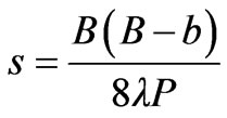
and . Notice that (2) and (3) do not include the path long error approximation increasing the accuracy of the results. The gain reduction factors can also be written as functions of the aperture phase error parameters in the Eand H-plane that are given by
 (4)
(4)
and
 (5)
(5)
respectively, as [6,17]
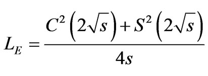 (6)
(6)
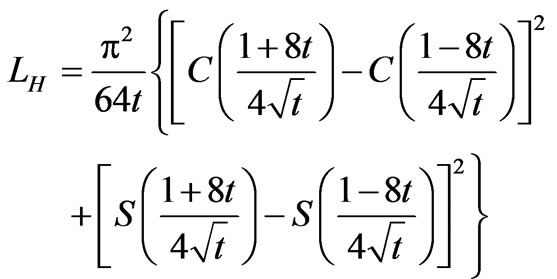 (7)
(7)
where  and
and  are the cosine and sine Fresnel integrals [23], respectively.
Equation (1) can be extended by incorporating the edge effect and the impact of the fringe currents at the aperture edges. In this case, the gain-formula becomes [5,7]
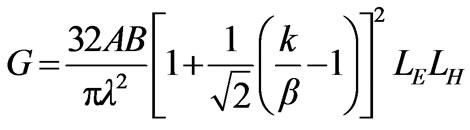 (8)
(8)
where  is the TE10 mode propagation constant [24]. The improved formula is valid for both pyramidal and sectoral horns. It reduces to (1) for large apertures (
 ) and calculates the gain values of the Eand H-plane sectoral horns by setting
  and
and , respectively.
3. Polynomial Description of the Gain Reduction Factors
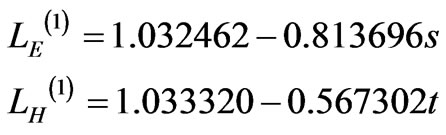
In [17], Aurand provided the following firstand secondorder approximations for the gain reduction factors:
 (9)
(9)
 (10)
(10)
that are valid for  and
and . Despite their accuracy in the given range of values, these approximations can not describe the gain reduction factors for phase errors far from the optimum gain condition ones (see next Section).
In this paper, we extend Aurand’s proposal and produce closed-form expressions for the gain reduction factors LE and LH by polynomial regression curve fitting [25-28] of (6) and (7). The fitting curves are linear polynomials calculated with the least squares method [25-27]. In this method, curve-fitting involves the minimization of the sum of the squared residuals, i.e. the squared differences between the exact LE (LH) value and the LE (LH) value that is computed from the curve-fit equation for the same aperture phase error. In order to get the best fit, we use the R2 goodness-of-fit statistics metric (this is the square of the sample correlation coefficient between the data values and the calculated ones from the fitting polynomial). The fit improves as R2 values approach unity.
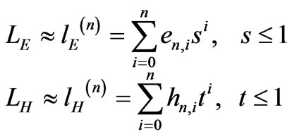
In practice, we approximate LE and LH with nth-order polynomials, i.e. it is
 (11)
(11)
Let en and hn be vectors with elements the polynomial coefficients en,i and hn,i, i = 0,1...n, respectively. In this case, we formulate the least squares problem as:
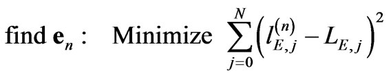 (12)
(12)
and
 (13)
(13)
The subscript j in (12) and (13) denotes that the specific values are calculated at s or t equal to  (the maximum value of the two aperture phase error parameters is one, see (11)). Each curve is evaluated at 10001 points in steps of 10-4 in the range [0,1], i.e. N = 104. Derivation of en and hn gives the nth-order polynomial approximation of LE and LH, respectively2.
Recall that the choice of the best fit approximation uses the R2 goodness-of-fit statistics metric. Table 1 gives the calculated R2 values for the best fit nth-order polynomial approximation of (6) and (7) for n = 1,2…10. The corresponding polynomial coefficients, en,i and hn,i, are given in Tables 2 and 3. In Table 1, we also give the F-statistic values [25-27] of each approximation (F-statistic value goes toward infinity as the fit becomes more ideal). Notice that LH is adequately approximated from a polynomial with order lower than the one that is required for LE. All the results were checked and validated using Matlab R2008a curve fitting routines [29].
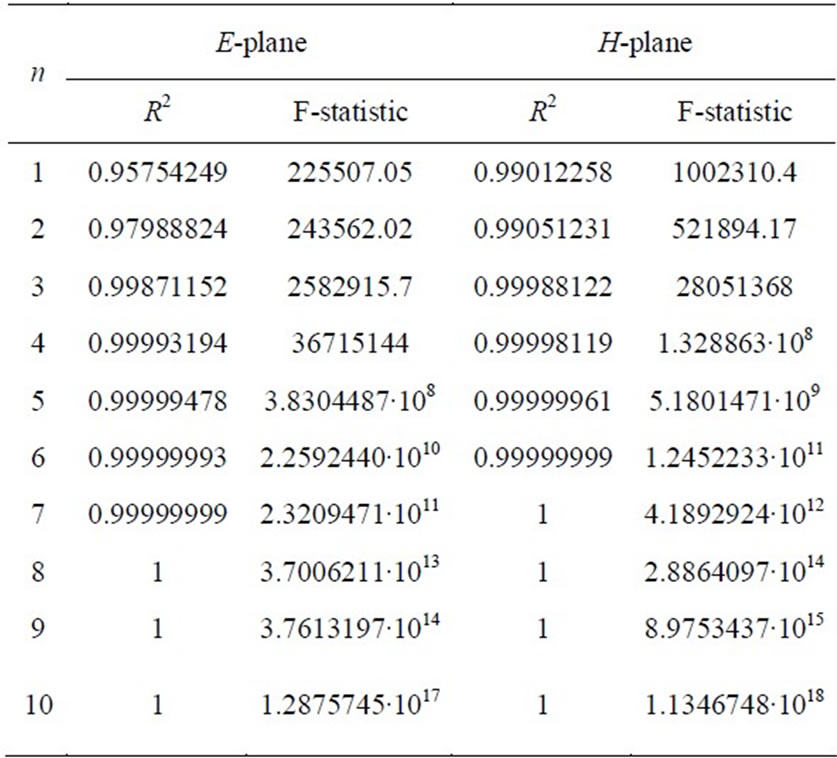
Table 1. Goodness-of-fit values
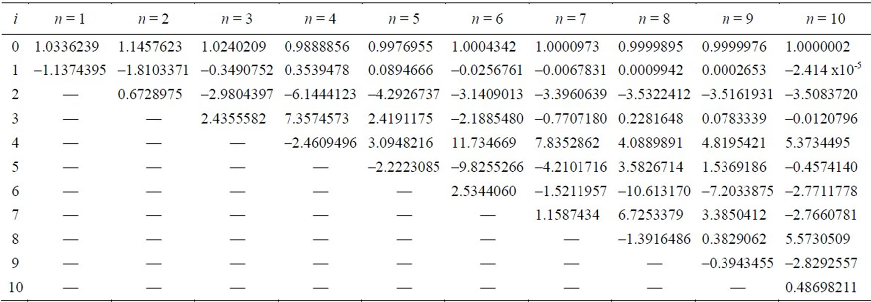
Table 2. Polynomial coefficients en,i

Table 3. Polynomial coefficients hn,i
In order to describe simple but accurately the gain reduction factor, we have to estimate the minimum required polynomial order. In practical terms, the goodness-of-fit statistics may not provide an efficient way to estimate the degree of error. In this case, a graphical inspection of the

Figure 3. E-plane gain reduction factor: Exact and approximate curves
fitting curves ensures the suitability of the proposed approximations. Figures 3 and 4 show the exact and the (approximate) fitting curves of the gain reduction factors. Notice that the curves that describe  and
and  are almost similar to the exact solution.

Figure 4. H-plane gain reduction factor: Exact and approximate curves
In order to further investigate the relation between the approximation error and the polynomial order, we used two well-known error metrics, the average absolute error and the rms error. Figure 5 shows the variation of the two metrics as a function of the polynomial order of the approximate formulas. We see that LH is adequately approximated with fewer terms than LE; for example,  and
and  yield errors less than 1%. We also notice that the average absolute error is always slightly smaller than the rms error.
4. Application Examples
In order to show the efficacy of our approach, we give three representative examples.
Example 1: Let us consider some typical X-band pyramidal horns, see Table 4. Horns operate at 10 GHz and they are fed from WR-90 waveguide. Their aperture phase errors are calculated from (4) and (5). Figure 6 illustrates the gain values of the horns. With G0,1 and G0,2 we present the values that are calculated from (1) using Aurand’s firstand second-order approximations, respectiveely; G1, G2, G4, and G6 are the results obtained from (1) and the proposed first-, second-, fourth-, and sixth-order approximation. G0 denotes the gain values that are calculated from (1) with adaptive quadrature integration of (2) and (3). Finally, Gacc are the exact gain values calculated with the professional antenna design software ORAMA [21].
As it was expected, (9) and (10) are adequate only for small values of s and t (moreover, G0,2 takes complex values for great values of s; these are not shown in Figure 6). In any case, the fourth-order approximations give results almost identical to the numerically calculated ones. The results are also in good consistency with the exact values calculated with ORAMA. The small gain values in cases 3 and 5 are due to the fact that the far-field gain is not maximized at the horn’s axis.
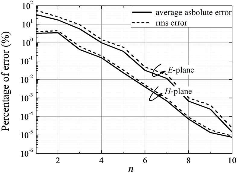
Figure 5. Average absolute and rms error versus the order of the fitting polynomials
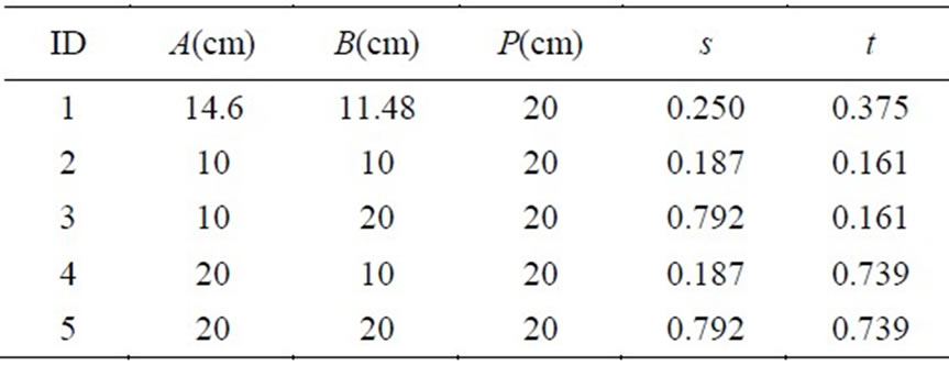
Table 4. Horns specifications
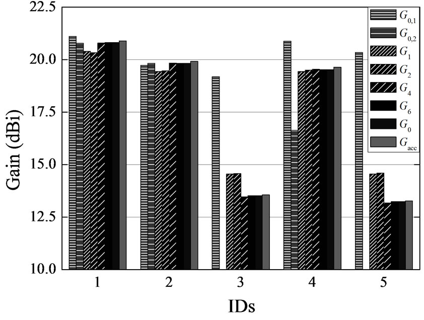
Figure 6. Calculated gain values (in dBi)
Example 2: We consider an Eand an H-plane sectoral horn that operate at 10 GHz and are fed from WR-90 waveguide. In the first case, B = 20 cm; in the second one, it is B = 20 cm. In both cases, the throat-to-aperture length is 20 cm.
First, we calculate the gain values from (8) with adaptive quadrature integration of (2) and (3). The exact horns’ gains are 9.1 dB (E-plane sectoral horn) and 10.15 dB (H-plane sectoral horn). The gain values that are obtained from (1) and (9) are 14.83 and 11.52 dB, respectively; Aurand’s second-order approximation gives worst results. On the other hand, our formulation gives (the subscript denotes the order of the fitting polynomial) that G1 = 10.19 dB, G2 = 10.22 dB, G4 = 9.03 dB and G6 = 9.09 dB (E-plane sectoral horn). In the case of the H-plane sectoral horn, the approximation error is smaller. The calculated gains are G1 = 10.37 dB, G2 = 10.39 dB, G4 = 10.15 dB, and G6 = 10.15 dB. Again, the fourthorder approximations give adequate results.
Example 3: In [11], Selvan proposed a design method for pyramidal horns of any desired gain and aperture phase error. However, the accuracy of his method is strictly related to the accuracy of the approximations of (6) and (7).
Let us consider the design examples in Table 5.
Table 6 gives the calculated horns dimensions with the method proposed in [11] using (10) (Aurand’s approximation) and the proposed second-, fourth-, and sixthorder approximations. Next, we used this data and calculated the exact gain values with ORAMA, see Table 7. Finally, Figure 7 shows the absolute relative error between the computed and the desired gain for each case. We notice that Aurand’s approximation is adequate at small values of s and t (IDs 1 and 3). However, as the aperture phase error parameters increase (IDs 2 and 4) these approximations lead to erroneous results. In any case, the proposal in [11] is an accurate design method when a polynomial approximation with polynomial order at least equal to four is used for the description of the gain reduction factors.
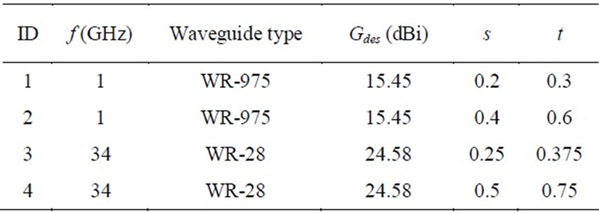
Table 5. Horns design examples
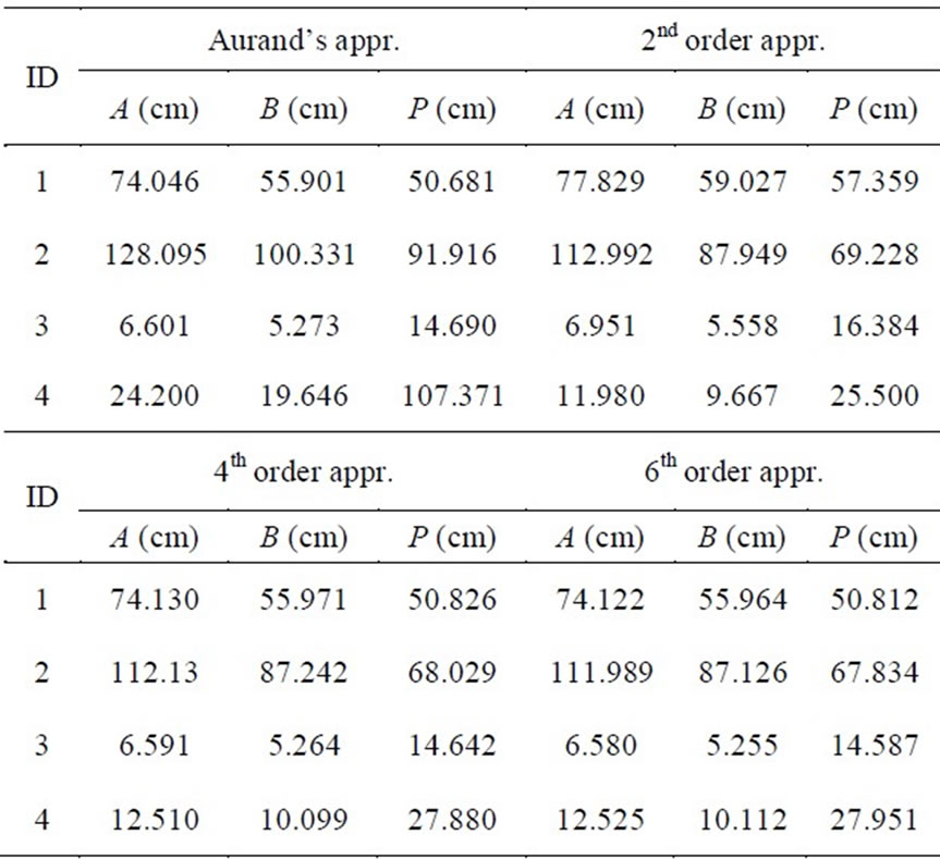
Table 6. Calculated hors dimensions
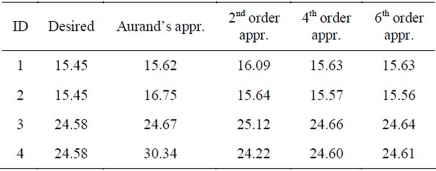
Table 7. Desired and calculated gain values (in dBi)

Figure 7. Relative gain errors
5. Conclusions
In this paper, we presented a set of nth-order polynomial approximate expressions for the gain reduction factors of pyramidal and sectoral microwave horns. The formulas were derived with polynomial regression curve fitting techniques. Comparisons with methods in the published literature and results calculated with commercial antenna design software verified the accuracy of the proposed formulation and demonstrated the benefits of the approach. We also explored the relation between the polynomial order of the derived formulas and the approximation error. It was found that that a third-order polynomial approximation of the gain reduction factor in the H-plane is adequate; in order to obtain accurate results in the E-plane, a fourth-order approximation is required. This paper extends previous work in the literature and applies to horns with large values of aperture phase errors. The proposed formulation is a useful tool in the analysis and design of rectangular horns, especially when simple closed-from expressions are required.
REFERENCES
- C. A. Balanis, “Antenna Theory: Analysis and Design,” 3rd Edition, John Wiley & Sons, Inc., Hoboken, 2005.
- S. A. Schelkunoff, “Electromagnetic Waves,” David Van Nostrand Company, Inc., New York, 1943.
- J. L. Teo and K. T. Selvan, “On the Optimum PyramidalHorn Design Methods,” International Journal of RF and Computer-Aided Engineering, Vol. 16, no. 6, November 2006, pp. 561-564.
- E. Jull, “Errors in the Predicted Gain of Pyramidal Horns,” IEEE Transactions on Antennas and Propagation, Vol. 21, no. 1, January 1973, pp. 25-31.
- K. T. Selvan, “An Approximate Generalization of Schelkunoff’s Horn-Gain Formulas,” IEEE Transactions on Antennas and Propagation, Vol. 47, no. 6, June 1999, pp. 1001-1004.
- G. Kordas, K. B. Baltzis, G. S. Miaris and J. N. Sahalos, “Pyramidal-Horn Design under Constraints on Half-Power Beamwidth,” IEEE Transactions on Antennas and Propagation, Vol. 44, no. 1, February 2002, pp. 102-108.
- K. T. Selvan, R. Sivaramakrishnan, K. R. Kini and D. R. Poddar, “Experimental Verification of the Generalized Schelkunoff’s Horn-Gain Formulas for Sectoral Horns,” IEEE Transactions on Antennas and Propagation, Vol. 50, no. 6, June 2002, pp. 875-877.
- K. Guney and N. Sarikaya, “Neural Computation of Wide Aperture Dimension of Optimum Gain Pyramidal Horn,” International Journal of Infrared and Millimeter Waves, Vol. 26, no. 7, July 2005, pp. 1043-1057.
- A. Akdagli and K. Guney, “New Wide-Aperture-Dimension Formula Obtained by Using a Particle Swarm Optimization for Optimum Gain Pyramidal Horns,” Microwave and Optical Technology Letters, Vol. 48, no. 6, June 2006, pp. 1201-1205.
- Y. Najjar, M. Moneer and N. Dib, “Design of Optimum Gain Pyramidal Horn with Improved Formulas Using Particle Swarm Optimization,” International Journal of RF and Computer-Aided Engineering, Vol. 17, no. 5, September 2007, pp. 505-511.
- K. T. Selvan, “Accurate Design Method for Pyramidal Horns of Any Desired Gain and Aperture Phase Error,” IEEE Antennas Wireless Propagation Letters, Vol. 7, 2008, pp. 31-32.
- W. T. Slayton, “Design and Calibration of Microwave Antenna Gain Standards,” Report 0594740, US Naval Research Laboratory, Washington, 1954.
- J. W. Odendaal, “Predicting Directivity of Standard-Gain Pyramidal-Horn Antennas,” IEEE Antennas and Propagation Magazine, Vol. 46, no. 4, August 2004, pp. 93-98.
- K. Harima, M. Sakasai and K. Fujii, “Determination of Gain for Pyramidal-Horn Antenna on Basis of Phase Center Location,” Proceedings of the 2008 IEEE International Symposium on Electromagnetic Compatibility-EMC 2008, Detroit, 18-22 August 2008, pp. 1-5.
- G. Mayhew-Ridgers, J. W. Odendaal and J. Joubert, “Improved Diffraction Model and Numerical Validation for Horn Antenna Gain Calculations,” International Journal of RF and Computer-Aided Engineering, Vol. 19, no. 6, November 2009, pp. 701-711.
- M. Ali and S. Sanyal, “A Finite Edge GTD Analysis of the H-Plane Horn Radiation Pattern,” IEEE Transactions on Antennas and Propagation, Vol. 58, no. 3, March 2010, pp. 969-973.
- J. F. Aurand, “Pyramidal Horns, Part I: Simple Expressions for Directivity as a Function of Aperture Phase Error,” Proceedings of the 1989 IEEE Antennas Propagation Society International Symposium, San Jose, Vol. 3, 1989, pp. 1435-1438.
- J. F. Aurand, “Pyramidal Horns, Part II: A Novel Design Method for Horns of Any Desired Gain and Aperture Phase Error,” Proceedings of the 1989 IEEE Antennas and Propagation Society International Symposium, San Jose, Vol. 3, 26-30 June 1989, pp. 1439-1442.
- T. Milligan, “Scales for Rectangular Horns,” IEEE Transactions on Antennas and Propagation, Vol. 42, no. 5, October 2000, pp. 79-83.
- T. A. Milligan, “Modern Antenna Design,” 2nd Edition, John Wiley & Sons, Inc., Hoboken, 2005.
- J. N. Sahalos, “Orthogonal Methods for Array Synthesis: Theory and the ORAMA Computer Tool,” John Wiley & Sons, Inc., Chichester, 2006.
- M. J. Maybell and P. S. Simon, “Pyramidal Horn Gain Calculation with Improved Accuracy,” IEEE Transactions on Antennas and Propagation, Vol. 41, no. 7, July 1993, pp. 884-889.
- E. W. Weisstein, “CRC Concise Encyclopedia of Mathematics,” 2nd Edition, Chapman & Hall/CRC, Boca Raton, 2002.
- D. M. Pozar, “Microwave Engineering,” 3rd Edition, John Wiley & Sons, Inc., New York, 2005.
- T. Hastie, R. Tibshirani and J. Friedman, “The Elements of Statistical Learning: Data Mining, Inference, and Prediction,” 2nd Edition, Springer, New York, 2008.
- J. Fox, “Applied Regression Analysis and Generalized Linear Models,” 2nd Edition, Sage Publications, Inc., Thousand Oaks, 2008.
- C. R. Rao, H. Toutenburg, S. Shalabh and C. Heumann, “Linear Models and Generalizations: Least Squares and Alternatives,” 3rd Edition, Springer, Berlin, 2009.
- F. Yang, J. Han, J. Yang and Z. Li, “Some Advances in the Application of Weathering and Cold-Formed Steel in Transmission Tower,” Journal of Electromagnetic Analysis and Applications, Vol. 1, no. 1, March 2009, pp. 24-30.
- A. Gilat and V. Subramaniam, “Numerical Methods for Engineers and Scientists: An Introduction with Applications Using MATLAB®,” 2nd Edition, John Wiley & Sons, Inc., Hoboken, 2010.
NOTES
1Usually, it is assumed that the overall efficiency (i.e. the product of the reflection, conduction, and dielectric efficiencies) of a rectangular horn is one. In this case, the on-axis far-field gain and the directivity of the horn are identical [1].
2A further discussion on this issue is beyond the scope of the paper; the interested reader can find additional information about the development and implementation of least squares algorithms in the proposed literature [25-27].