Journal of Electromagnetic Analysis and Applications
Vol. 2 No. 3 (2010) , Article ID: 1540 , 6 pages DOI:10.4236/jemaa.2010.23021
Analysis of the Electromagnetic Pollution for a Pilot Region in Turkey
![]()
Faculty of Engineering and Architecture, Department of Electrical and Electronics Engineering, Selçuk University, Konya, Turkey.
Email: eryaldiz@gmail.com, ozgurgenctr@yahoo.com
Received November 10th, 2009; revised December 11th, 2009; accepted December 15th, 2009.
Keywords: Electromagnetic Pollution, Statistical Analysis, Electromagnetic Radiation
ABSTRACT
In this paper, electromagnetic (EM) pollution (or radiation) measurements in a transmitter region were performed and statistical analysis of values recorded for the EM sources causing pollution was carried out. The actual measurement values and the estimated values by the analysis model obtained through the statistical analysis were compared. EM radiation levels were measured in the districts of Turkish capital Ankara where cellular base stations and TV/Radio stations are densely populated. EM Radiation (EMR) levels were measured for the GSM900, GSM1800, UHF4, VHF4 and VHF5 stations for certain spectrum ranges under far-field conditions by utilizing isotropic field probe and selective spectrum analyzer. The obtained measurement levels were compared with the limit values given by International Commission for Non-Ionizing Radiation Protection (ICNIRP). The results are discussed, regarding both the obtained values that influence the measurements.
1. Introduction
The use of EMR for communication increased significantly in the recent years (radio, television and cellular) and consequently the environmental level of EMR has increased. The massive proliferation of mobile communications equipment raised a special concern regarding the safety of population and personnel exposed to radiofrequency (RF) radiation emitted by either the base-station antennas [1].
The potential health effects of EMR from the transmitters for broadcasting of radio/TV and mobile communication are the subject of on-going researches [2,3] and a significant amount of public debate. The distribution and levels of EM pollution in the crowded residential areas are very important.
Exposure standards for RF region of EM spectrum, applicable at national or international level give for the UHF and VHF band of interest the RMS electric field strength maximum accepted values as reference levels for occupational or population exposure [1] in the far field region of the sources.
EM pollution measurements within the scope of this study were executed in a chosen pilot region, the city centre of Ankara, Turkey. The measurements were specifically in Dikmen Caldagi Hill transmitter region where many EM pollution sources are located.
In the present, there are three public mobile communication operators in Turkey: Vodafone (GSM 900 MHz), Turkcell (GSM 900 MHz), AVEA (GSM 1800 MHz or DCS 1800 MHz).
From the statistical analysis of the measurement results, EM radiation levels can be modeled through various calculations and formulas retrieved under certain conditions and within acceptable correctness. EM pollution measurement results are examined by means of time series analysis whether these results are suitable for predicting through the created model. Estimation or determination of the dependant variable total EM pollution is realized as based on the modeling.
2. Measurement of EM Pollution
In this EM pollution measurement study; it is assumed that only far field conditions exist for the cellular (GSM900 and GSM1800), TV and radio transmitters since these installations are most of the time mounted on high towers or hills.
It is essential to measure the combined field levels for all different signal sources in the environment like as shown Figure 1. In practice, many of the directional antennas with high gains are not suitable for this purpose since they don’t allow measurements of signals from all directions and different polarizations and therefore not
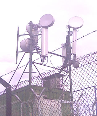
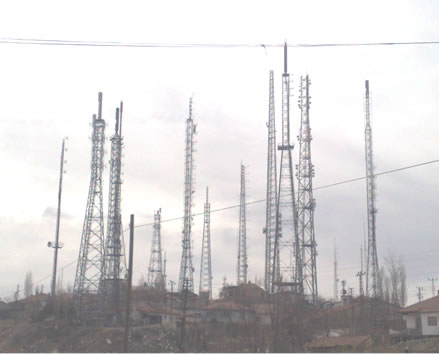
Figure 1. Some EM pollution sources in the measurement areas
allowing quick measurements. The system we used is designed for measurements of the E-field strength. This ensures that optimum settings are used and allows evaluation according to single frequencies, complete services and total emission. Since the tri-axis sensor (antenna) has got an isotropic characteristic, the measurement is done independent from direction or polarization of the emitter [1].
In the measurements, the wide band spectrum (75 MHz – 3 GHz) antenna probes that can measure from all directions and different polarizations [4,5,6] were used.
The measurements were fulfilled by using NARDA SRM3000 radiation meter with isotropic antenna that can be utilized in 75 MHz – 3 GHz frequency range. The measurement system comprises of an isotropic broad band antenna that is connected via combiner to a portable spectrum analyzer. The electric field probe was based at 2m height from the ground level. The EMR meter was interfaced with a portable computer. Measurement results recorded by using SRM3000 were saved to a computer [5]. Random measurements were performed in the transmitter region, far from GSM base station and radio/TV transmitters in far-field points. The antenna was mounted on a tripod. The signal from the EMR meter is expressed in Volt units convertible to electric field strengths (V/m) using the antenna factor parameter. All measurements were divided according to their relevant frequencies into groups (Radio, TV, Cellular, etc). For each measurement Eaverage (V/m) was recorded [8]. The duration of each measurement was 6 minutes [7,8]. The experimental set-up is depicted in Figure 2.
The measurements include the sources listed in Table 1 and the other sources within the spectrum up to 3 GHz.
3. Statistical Analysis of EM Pollution Measurements
The measurement results are analyzed by means of the SPSS 17.0 and E-views software. Firstly, stability of the obtained time series was examined using Dickey-Fuller (D-F) test in order to determine if the time series are suitable for estimation. In the second stage, the relationship between the variables was examined using correlation and regression analyses. Finally, variance analysis
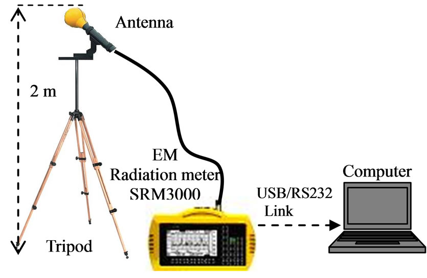
Figure 2. Equipment used for the measurements
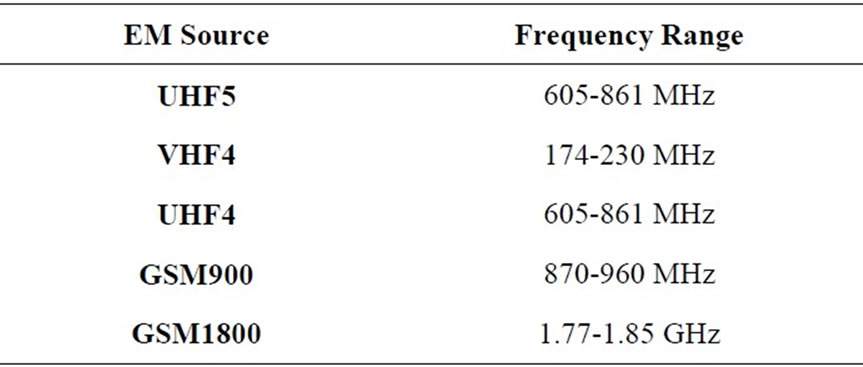
Table 1. Measured EM pollution sources and their frequency ranges
was utilized to determine the model’s significance and the prediction model for total EM pollution was obtained.
A time series is a group of measurement results recorded over a time for a certain variable in hand. The purpose of this analysis related to time series is to understand the reality represented by the observation set and determination of the predicted values of the variables in the time series. First step of predicting is to test the stability of the series. If the average or variance of the time series does not present a symmetrical change or the series is free of periodical fluctuations, these series are called “stable time series” [9]. D-F test is utilized for stability tests.
3.1 Dickey-Fuller Unit Root Test
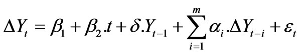
Unit root test analyses are applied for each time series of different measurement variables (GSM900, GSM1800, etc.) by using Equation (1) which is also utilized when testing the stability of series using D-F test [10].
 (1)
(1)
In Equation.1, Δ is the first difference processor and represents the difference between two consecutive values. Here, εt is the consecutive independent probable error term with zero average and unchanged σ2 variance and conforms to classic assumptions. δ=ρ-1 and ρ is a significance coefficient. If ρ=1, then constant of Yt-1 becomes zero and this indicates that the time series is unstable meaning that it does not have a unit root. β1 is a constant and β2 is the coefficient at t time. t represents trend and m is maximum delay [9,10]. Whether the series has a unit root while using D-F test or not are determined by trying the following hypothesis.
H0: ρ = 1 or δ = 0 (Series has unit root, are not stable)
H1: ρ < 1 or δ < 0 (Series does not have unit root, are stable).
Critical values for testing stability are the τ statistical values calculated by the D-F method. Acceptable limits (critical values) of this test according to the 5% level are calculated according to the Monte Carlo Simulation by MacKinnon. These values are called MacKinnon critical values. Known t statistics calculated by the statistical analysis programs are called τ statistics or D-F test statistics in this hypothesis test [10].
If the D-F test statistics’ absolute values are smaller than the MacKinnon Critical Values’ absolute values, H0 hypothesis is accepted and this indicates that the series is not stable. If the D-F tests statistics’ absolute values are greater than the MacKinnon Critical Values’ absolute values, H0 hypothesis is rejected and this indicates that the series is stable. If the original state of the series is not stable, first difference of the series is taken and the D-F test is applied again. If this is also not stable, second difference of the series is taken and the D-F test is re-applied [9,10].
According to the results in Table 2; when examined the values of each series, absolute values of τ statistics are greater than the absolute values of the critical values at 5% significance level. Therefore, the H0 hypothesis is rejected for the level values of each series examined [9]. In other words, all of the series (Total, GSM900, etc.) do not have unit root at level and are called stable. Using these data multiple regression can be utilized and future predictions can be made.
3.2 Regression and Correlation Analysis
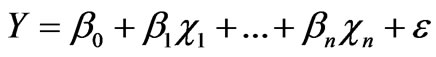
Regression analysis is an analysis method used to examine the relation between a dependant variable and one or more independent variables [11]. With multiple regression the relation between a dependant variable Y and more than one independent variables (X1, X2, …, Xn) is examined (Equation (2)).
Multiple Linear Regression Model: If Y is total EM pollution value, multiple linear regression model is given by
 (2)
(2)
where  is a constant,
  is the correlation coefficient of 1st variable,
  is the actual measurement value of the 1st variable, and
  is the error term.
The slope direction and the degree of the relationship among the variables contributing to the EM pollution in the environment are examined analytically by means of the correlation test and comparisons of the variable pairs. The influences of variables to each other are analyzed as shown in Table 4 for this study.
As shown in Table 3, total pollution value was recorded average 3.658 V/m and its standard deviation was 0.538 according to the 68 measurement results taken from various locations in the city centre. GSM1800 average pollution value was calculated 1.276 V/m while GSM900 average pollution value was 0.102 V/m.
According to Table 4, VHF4 was found being the highest correlation relation of 0.606 with total variable. UHF5 was the second highest variable with correlation of 0.583.
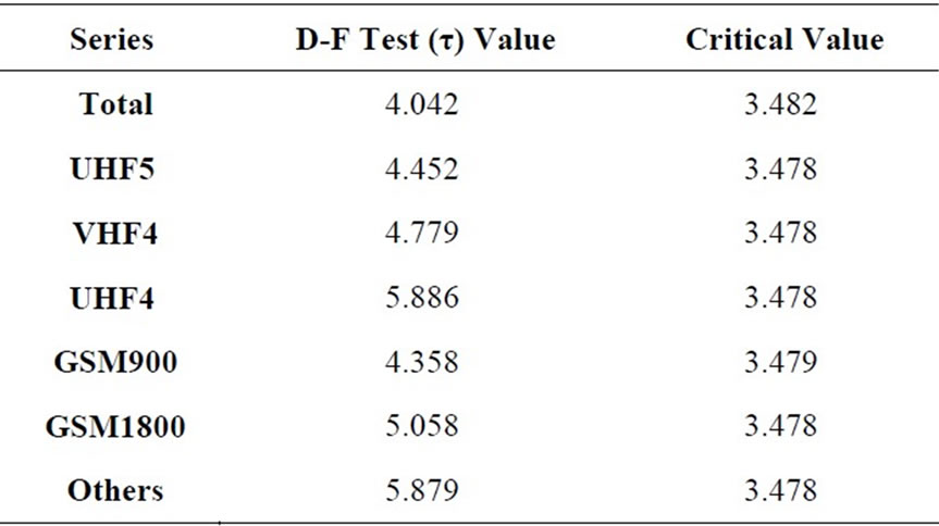
Table 2. D-F unit root test results for series
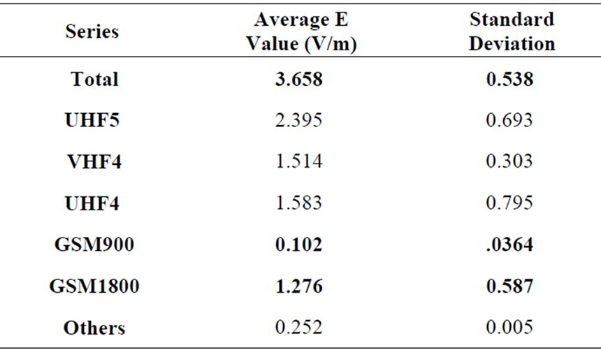
Table 3. Descriptive statistics related to the variables
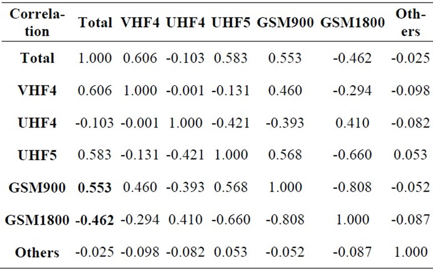
Table 4. Correlation related to the variables
Functional form of the relation between the variables is examined using regression analysis and its reliability degree is determined using correlation analysis. In Table 5, R2 multiple certainties factor and corrected multiple certainty factor R2corrected are used to determine the best regression model.
Model’s explanation strength is determined using the R2 multiple certainty factor. R2 value is a measure indicating what percentage of the total variation of a dependant variable can be explained by variations of the independent variables [11].
Durbin Watson test is utilized while testing the assumption of successive dependency (autocorrelation) between the data set observations requirement in order to apply the multiple linear regression method. R2 which is an indication of how good the independent variables describe the dependant variable was 92.7% (0.927) meaning that the EM pollution changes by 92.7% depending on these factors. R2 increases by adding more variables to the model, but this alone is not sufficient for testing the significance of the model. If the Durbin Watson Value is between 1.5 and 2.5, then autocorrelation does not exist and the prediction model is considered as deterministic [10]. Durbin Watson test statistics being 2.003 indicates absence of autocorrelation.
3.3 Variance Analysis and t Test
Significance column value (or p value) of variance analysis table (Table 6) indicates that the relationship between the variables is statistically significant if it is at (p < 0.05) level. The model’s overall significance is tested by F test [9]. Hypothesis:
H0: Coefficients are greater than 0.05. The model is not significant.
H1: Coefficients are little than 0.05. The model is significant.
If the relationship in Table 6 is formulized, the probability value F calculated according to p = 0.05 is

Table 5. Regression model summary for significance test
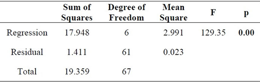
Table 6. Variance analysis p = 0.000 < 0.05, then the H0 hypothesis is rejected and the model is called to be significant.
The test is applied for significance of the coefficients in the regression model and the insignificant values are taken off from the model. For this purpose, t test is applied. When the t values which calculated according to p = 0.05 in Table 7 are tested, the H0 hypothesis is rejected for each coefficient.
H0: Regression coefficients are greater than 0.05. Relationship is not significant.
H1: Regression coefficients are little than 0.05. Relationship is significant.
Whether the significance level of independent variables is sufficient for the model or not is decided by looking at the p probability values. If p < 0.05, then the variable effects the dependent variable and is included to the model, otherwise it is assumed that it does not statistically effect the dependent variable and is not included in the model [9].
According to the results retrieved from the environmental measurements values, since the probability values (p values) of VHF4, UHF4, UHF5 and GSM1800 variables are smaller than 0.05, they are included to the
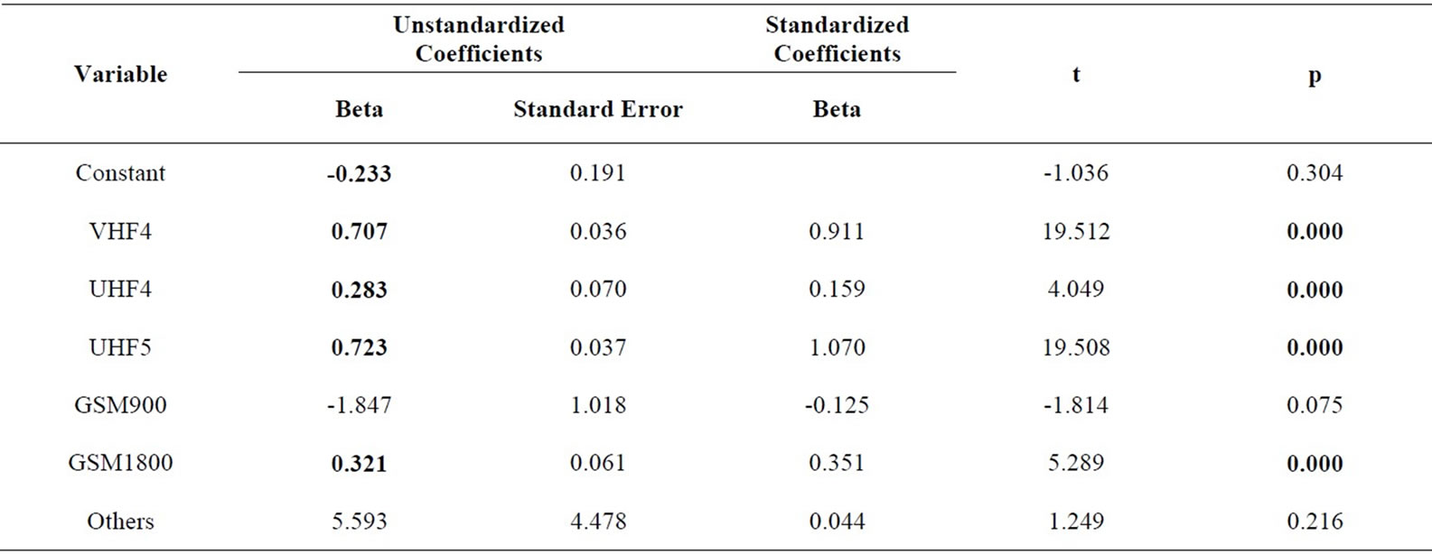
Table 7. Variable coefficients for EM pollution analysis model
model, but it is concluded that the GSM900 and Others variables are not significant for the model. As shown in Table 7, GSM900 and Others variables’ p probability values are respectively 0.75, 0.216 and are greater than 0.05. Hence, they can not be included to the prediction model. The multiple regression model is obtained as the following:
Total EM pollution value = -0.233 + 0,707.VHF4 +
0,283.UHF4 + 0,723.UHF5 + 0,321.GSM1800(3)
The independent variables that affect the total variable were tested using the multiple linear regression analysis, were included to the model, and were studied. According to the data collected during the measurements, the effect of VHF4 frequencies to the overall total pollution is around 0.707. The effect of UHF4 to the total pollution is 0.283, UHF5 is 0.723, GSM1800 is 0.321.
It is necessary that the errors are distributed normally in order to the obtained model to be significant. It is concluded that the distribution of the total pollution errors are normal since the measurement values are scattered around a 45o linear line when tested with the Probability-Probability (P-P) graphics method. A probability plot is a graphical technique for comparing two data sets, either two sets of empirical observations, one empirical set against a theoretical set, or more rarely two theoretical sets against each other [12,13]. Distribution of the values for the estimated regression models is shown in Figure 3.
The estimated model is valid when the observed and expected values’ distribution is examined.
3.4 Comparison of the Measurement Results by Means of Statistical Model
As a result of the D-F unit root tests applied to the measurements taken from the measurement region in general, the H0 hypothesis is rejected for level values of each series examined (as shown in Table 8). This indicates that the series do not have unit root at the level and are stable. Consequently, it is possible to utilize multiple regressions using the obtained results and it is concluded that predictions for future can be made.
The calculated value by the model (Equation (3) is 3.96 V/m while the actual total pollution value is 4.094 V/m (as shown in Table 8). Hence, the prediction model is significant and valid when examined the observed and predicted values’ distribution. Having valid models obtained for the measurement regions indicates that the EM pollution values are suitable for prediction future pollution levels. The studies indicated that very close values are recorded when compared the prediction result of the model obtained from the analysis made by using the SPSS17.0 analysis program and the actual measurement results.
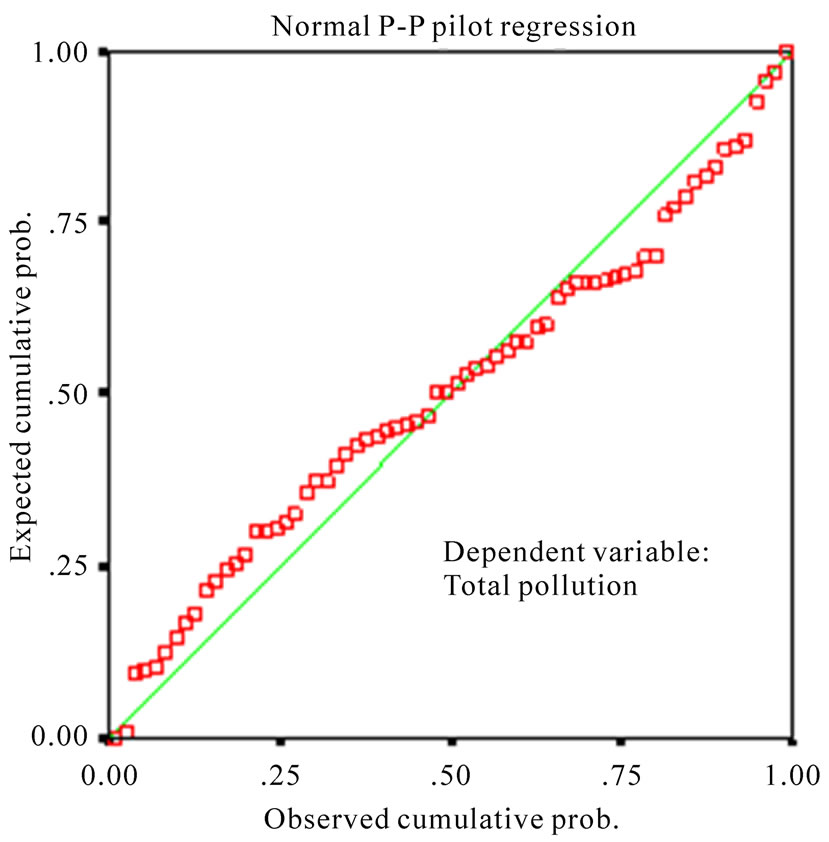
Figure 3. Observed and expected cumulative probability graphics for total EM pollution
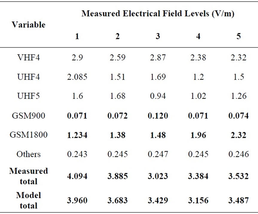
Table 8. Sample comparison of environmental measurement results
4. Conclusions
The study involved 68 measurements to determine the EM field levels in Dikmen Caldagi Hill transmitter region in the Ankara city centre. The precise experimental determination of E-field of RF radiation in a complex environment is a difficult task. This is mainly due to the existence of three fundamental physical properties of electromagnetic waves: reflection, absorption and interference. Under uncontrolled conditions, for instance in a complicated environment, different measurements can lead to quite different results due to changing conditions. Moreover, the settings of the measurement equipment may affect sensible the measured values [1].
As shown in Table 3, total pollution value was recorded as average 3.658 V/m and its standard deviation was 0.538 according to the 68 measurement results taken from various locations in the city centre. GSM1800 average pollution value was calculated as 1.276 V/m and its standard deviation was calculated 0.587. GSM900 average pollution value was 0.102 V/m and its standard deviation was calculated 0.0364. The electric field level of GSM900 base stations were measured maximum 0.483 V/m and minimum 0.078 V/m during the measurements. For GSM1800, maximum 2.32 V/m and minimum 0.09 V/m electric field levels were measured. Average total pollution values were measured as maximum 5.21 V/m and minimum 2.53 V/m. VHF4 average pollution value was found being the highest correlation relation of 0.606 with total EM pollution value. GSM900 average pollution value was found 0.553 correlation relation with total value. In other words, total EM pollution is affected by 55.3% due to variation in pollution of GSM900 and by 46.2% for GSM1800.
Results indicated that the EM pollution levels were below the 41.25 V/m limit for 900 MHz and 58.34 V/m limit for 1800 MHz according to ICNIRP’s recommendations [14].
REFERENCES
- S. Miclausi and P. Bechet, “Estimated and measured values of the RF radiation power density around cellular base stations,” Environment Physics, Bucharest, Vol. 52, No. 3, pp. 429–440, 2007.
- B. I. Wu, A. I. Cox, and J. A. Kong, “Experimental methodology for non-thermal effects of electromagnetic radiation on biologics,” Journal of Electromagnetic Waves and Applications, Vol. 21, No. 4, pp. 533–548, 2007.
- C. Giliberti, F. Boella, et al., “Electromagnetic mapping of urban areas: The example of Monselice (Italy),” PIERS Online, Vol. 5, No. 1, pp. 56–60, 2009.
- A. R. Ozdemir, “Radio frequency electromagnetic fields levels in urban areas of Istanbul, Ankara and Izmir and protection techniques,” Thesis for Expertise, Telecommunication Society, Ankara, Turkey, 2004.
- A. Shachar, R. Hareuveny, M. Margaliot, and G. Shani, “Measurements and analysis of environmental radio frequency electromagnetic radiation in various locations in Israel,” Soreq Nuclear Research Center, Israel, 2004.
- K. Voudouris and P. Grammatikakis, “Radiation measurements at short wave antenna park,” Department of Electronic, Technological Educational Institute of Athens, Athens, 2005.
- R. Hamid, M. Cetintas, et al., “Measurement of electromagnetic radiation from GSM base stations,” IEEE International Symposium on EMC, TUBITAK-UME, Gebze, 2003.
- P. Getsov, D. Teodosiev, et al., “Methods for monitoring electromagnetic pollution in the Western Balkan environment,” SENS’2007, 3rd Scientific Conference with International Participation Space, Ecology, Nanotechnology, Safety, Varna, 2007.
- D. Gujarati, “Basic econometrics,” Literature Publishing, Turkey, 2001.
- M. Sevuktekin and M. Nargelecekenler, “Time series analysis,” Nobel Publishing, Turkey, 2005.
- H. Emec, “Time series econometry I: Stability, unit roots,” IIBF, Dokuz Eylul University, Izmir, 2007.
- H. C. Thode, “Methods of probability plotting,” CRC Press, 2006.
- J. Gibbons and S. Chakraborti, “Nonparametric statistical inference,” 4th Ed., CRC Press, 2003.
- ICNIRP, “Guidelines for limiting exposure to time-varying electric, magnetic and electromagnetic fields (up to 300 GHz),” Health Physics, Vol. 74, No. 4, pp. 494–522, 1998.