Int'l J. of Communications, Network and System Sciences
Vol.6 No.4(2013), Article ID:30382,11 pages DOI:10.4236/ijcns.2013.64022
Fractal Model of Rocks—A Useful Model for the Calculation of Petrophysical Parameters
Council for Geoscience, Pretoria, South Africa
Email: valeriya@geoscience.org.za
Copyright © 2013 V. Yu. Hallbauer-Zadorozhnaya. This is an open access article distributed under the Creative Commons Attribution License, which permits unrestricted use, distribution, and reproduction in any medium, provided the original work is properly cited.
Received August 15, 2012; revised September 30, 2012; accepted October 25, 2012
Keywords: Fractal; Sediments; Resistivity; Porosity; Permeability
ABSTRACT
A fractal model containing n-series of spheres and ellipses with corresponding radii, and surrounded by a thin film of adsorbed water has been developed. This model is more suitable to real sedimentary rocks because it not only allows for varying grain sizes and number of fractions, but also takes into consideration the influence of double electrical layers on the physical properties of sediments. Ellipsoid fractal models provide mathematical proof of the phenomenon of supercapillary conductivity observed in laboratory measurements. Using the parameters of the fractal models several petrophysical parameters can be calculated, namely resistivity porosity, and permeability. In a case study, layers with different resistivity were identified on a section taken from a TDEM survey, and porosity and salinity of water bearing layers were estimated using the fractal model. Estimated permeability using the fractal model showed good agreement with other methods.
1. Introduction
For many years determining the resistivity of layers was deemed a significant result of applied EM geophysics. However, problems intended to be solved by geophysics have become more complex. Now electromagnetic methods are aimed at defining other petrophysical parameters such as porosity, permeability, polarization parameters, oil and gas saturation etc. Therefore a new model for mathematical modeling of petrophysical parameters is required.
There are a number of factors that must be taken into account when creating this model. It is well known that resistivity decreases with increasing porosity of sediments. However, components filling the pore spaces of rocks considerably influence the petrophysical parameters of rocks. In addition, rocks/sediments can be regarded as two component aggregates, i.e. matrix and fluid, where fluid can be water, gas and/or a mixture of them. Rocks or sediments can also be composed of three component aggregates (matrix-clay-fluid/gas). Moreover, for many cases the influence of double electrical layers (DEL) surrounding grains of sediments must be taken into account when calculating resistivity.
There are numerous experimental works looking at the interdependence of porosity and resistivity of sediments of different kinds and different ages. However, there is insufficient application of these theoretical considerations to the interpretation of electromagnetic data and physical modelling of data. Traditionally for many years the empirical Archie’s law [1] has been used for interpreting EM data. It allows for the estimation of the porosity of sediments if the dependence between resistivity and porosity (at least the structural index of porosity) is known. Nearly two thirds of a century has passed since this law was formulated, and our knowledge of the sediment structure has improved, however, the empirical Archie’s law is still widely used, and other considerations have seldom been applied for interpreting EM and laboratory measurement data. It should be noted that the geometrical factor of Archie’s law is based on the specific kind of sediments in question:
 (1)
(1)
where ![]() is a coefficient that is dependent on the kind of sediments and can be in the range 0.4 -> 1, φ is the porosity of sediments (dimensionless unit) and m is an index of tortuosity of the pore channels which can be in the range 1.3 - 2.2 or greater [2]. The structures of pores which make up solids are very complex and are unique for each kind of sediment. Obviously, if there is no trustworthy data for the resistivity of sediments in a study area, the interpretation becomes a gamble. The problem becomes underdetermined, with one resistivity value and three unknown parameters (α, φ and m). Moreover Archie’s model also does not take into account the influence of double electrical layers, although it has been shown (as shown by [3]) that for specific cases the electrical resistivity of clay can be twice as low as when water fills the pore space of the clay. It is also known that the DEL are responsible for different kinds of induced polarization effects that arise in sediments due to applied electrical currents and also influence the measured resistivity.
is a coefficient that is dependent on the kind of sediments and can be in the range 0.4 -> 1, φ is the porosity of sediments (dimensionless unit) and m is an index of tortuosity of the pore channels which can be in the range 1.3 - 2.2 or greater [2]. The structures of pores which make up solids are very complex and are unique for each kind of sediment. Obviously, if there is no trustworthy data for the resistivity of sediments in a study area, the interpretation becomes a gamble. The problem becomes underdetermined, with one resistivity value and three unknown parameters (α, φ and m). Moreover Archie’s model also does not take into account the influence of double electrical layers, although it has been shown (as shown by [3]) that for specific cases the electrical resistivity of clay can be twice as low as when water fills the pore space of the clay. It is also known that the DEL are responsible for different kinds of induced polarization effects that arise in sediments due to applied electrical currents and also influence the measured resistivity.
Another way to calculate resistivity that shall be used for this study is by way of mathematical modelling of petrophysical properties using matrix (fractal) models. It appears that the first person to introduce the fractal model in petrophysics in 1948 was A. S. Semenov [4], with furtherpositive results being obtained by Pape et al. [5]. Following this author a matrix (fractal) model has been proposed for this study. A fractal modelcontaining n-series of spheres and ellipses with corresponding radii and surrounded by a thin film of adsorbed water (DEL) has been used. This model is more suitable for real sedimentary rocks. Using the parameters of the fractal model several petrophysical parameters can be calculated namely: resistivity, total and effective porosity and permeability.
2. Matrix Model of Sediments
Usually the solid part of sediments consists of a mixture of polymineral grains. They are naturally dielectric with high resistivity values reaching up to 10−11 Ωm and more (ρ1). The second component of sediments is fluid or a mixture of material filling the pore spaces, such as fluid and clay (ρ2). More seldom (in the case of ore) the second component is presented by conductors or semi-conductors with very low resistivity. It follows then that the resistivity of sediments/rocks (ρ1,2) depends on the values of ρ1 and ρ2; on the relative volume of components V1 and V2, whereV2 = (1 − V1); and on the form and distribution of dielectrics and conductors in the solid. The dependence of ρ1,2 on ρ1 and ρ2can be presented as [6]:
 (2)
(2)
where PP is a parameter of porosity (or structural factor) which is the ratio of the resistivity of the sediment to the resistivity of the material filling the pore spaces.
The dependence of ρ1,2 on ρ1 and ρ2 were studied both experimentally and theoretically for different kinds of rocks/sediments. For the theoretical investigation, the solids were presented as simplified matrix models. The matrix models can be regarded as uniformly distributed packages of identical sizes or different sizes. The packages can be spheres, cubes, ellipsoids, cuboectaedres, rectangles, planes and other geometrical figures. The pore space is filled by a second component, such as water, clay, water/clay, or metal. Table 1 shows some of the equations used for calculating ρ1,2 using different matrix models.
2.1. Double Electrical Layers
It must be noted that only the model introduced by Semenov take into account different sizes of solid particles. However even this model does not take note of the existence of double electrical layers (DEL), which are known to be associated with the interface between minerals and pore fluids. Figure 1 is a schematic representation of Stern-Gouy’s model of DEL.
The DEL can be regarded as consisting of two regions, namely an inner region or dense part where ions are adsorbed onto the solid surface through electrostatic and Van der Waal’s forces (the Stern layer); and an outer or diffuse region where ions are under the combined influence of the ordering electrical and disordering thermal forces (the Gouy layer). Therefore, two planes can be distinguished in the DEL, namely an inner plane, which is the surface of the solid, and an outer diffuse plane.
The thickness of the dense part of the DEL is approximately σ0del = 10−9 [7]. The thickness of the diffuse layer depends on the concentration of the electrolyte. If the thickness of the diffuse layer is less than σ0del then the electrolyte is concentrated. Otherwise if 
Table 1. Equations that allow for the calculation of ρ1,2 using different two component matrix models, assuming  and
and  is low (after Kobranova, 1984, [2]).
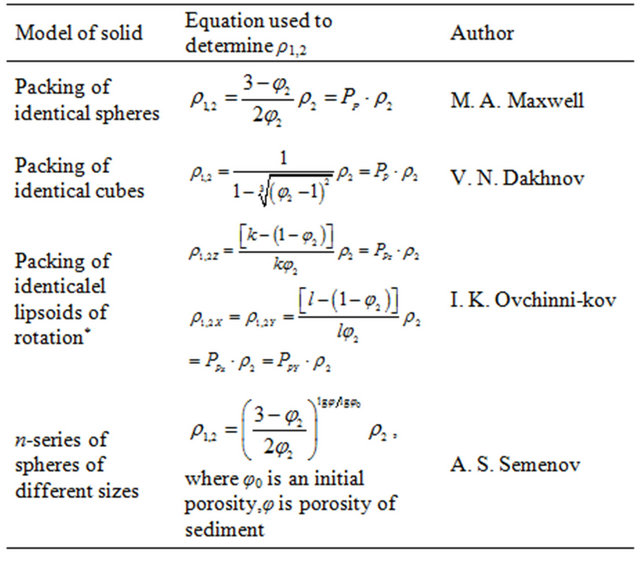
*where k and l are coefficients of form, which change from k → 0 and l → for avery oplate ellipsoid of rotation, up to k →
 and k → −1 for avery prolate ellipsoid of rotation. For spherical grains k = l = −2.
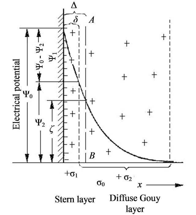
Figure 1. A schematic representation of Stern-Gouy model of double electric layer.
the electrolyte is regarded as diluted. For a 1:1 valence electrolyte the boundary between concentrated and diluted is accepted as C = 0.1 N. In the case of concentrated electrolytes the electrokinetic phenomena is suppressed. A characteristic thickness of the diffusion part of the DEL σdel can be described as [7]
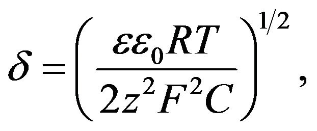 (3)
(3)
where ε is dielectric permeability, ε0 is the electrical constant, R is the gas constant, T is the absolute temperature, F is the Faraday number, z is the valence of the ions and C is the concentration of electrolyte (mol). Note the thickness of the DEL σdel indicates the distance where the transfer number of cations Cc and anions Ca are noticeably different. The thickness of the DEL ranges from a few nanometres up to hundreds of micrometres. If the concentration of the electrolyte NaCl is 0.01 N (0.56 g/l), the thickness of the DEL is equal to 3e−9 m. If the concentration of the electrolyte NaCl is 0.001 N the thickness of the DEL is equal to 1e−8 m.
2.2. Structure of Sediments as a Fractal
For this study, the most applicable model for clastic sediments is the model introduced by A. S. Semenov. This model contains n-series of spheres of different sizes. Let us assume the resistivity of the matrix is very high and the second component of the model is water with resistivity ρf. Following [4] let us also assume that the first volume fraction is represented by the biggest grains occupying volume V0 and the rest of the volume φ0 = (1 ‒ V0) is occupied by a series of smaller grains. The second fraction of smaller grains will occupy a volume (1 ‒ V0)· V0. The third fraction of even smaller grains will occupy a volume (1 ‒ V0)2·V0, etc. The rest of the volume (1 ‒ V0)n will be equal to the porosity coefficient of the sedimentφ. Obviously the coefficient of porosity φ will be determined by the fraction of spherical grains n. The resistivity of this model is equal to:
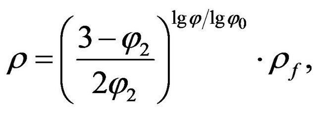 (4)
(4)
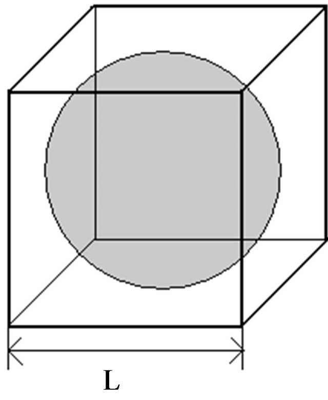
Let us consider the case for one unit of the medium - a cube with size L = 1, and include into this cube a sphere with radius r1 = L/2 = 0.5 (Figure 2(a)). The volume of this sphere is V1. This sphere will be regarded as a main grain (grain of the first fraction). The rest of the volume (porosity coefficient) will then be equal to
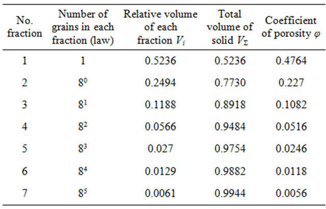
 . (The most widely used physical unit of porosity is percent; however it can also be presented as a dimensionless unit. Therefore, the dimensionless unit can refer both to porosity and the coefficient of porosity). This model is very often used for description of sediments structure although the porosity of a package of identically sized spheres described by Maxwell’s formula (Table 1) is equal to 0.4764. This model containing the fracture of only one size is suitable to describing well sorted sands and bioherm and limestones only.
The third fraction occupies the volume  Grains of this fractionare located on the corners of the cubes which include the grains of the second fraction (Figure 2(b)). The radius of the grains of the third fraction r3 = 0.1503. It follows then that the total volume of the solid is equal to V1+2+3 = 0.8918 and the volume of the pore space is equal to φ = 0.1082.
Continuing in this way, we obtain the parameters of the fractal model which are presented in Table 2.
The table shows the dependence of the porosity coefficient (porosity) on the number of fractions of different size (in the solid. When these calculations are applied to a model containing grains of such a size such that the thickness of the DEL is negligible compared to the radii of all spheres, the effective and dynamic porosity of the sediment will equal the total porosity.
 (a)
(a)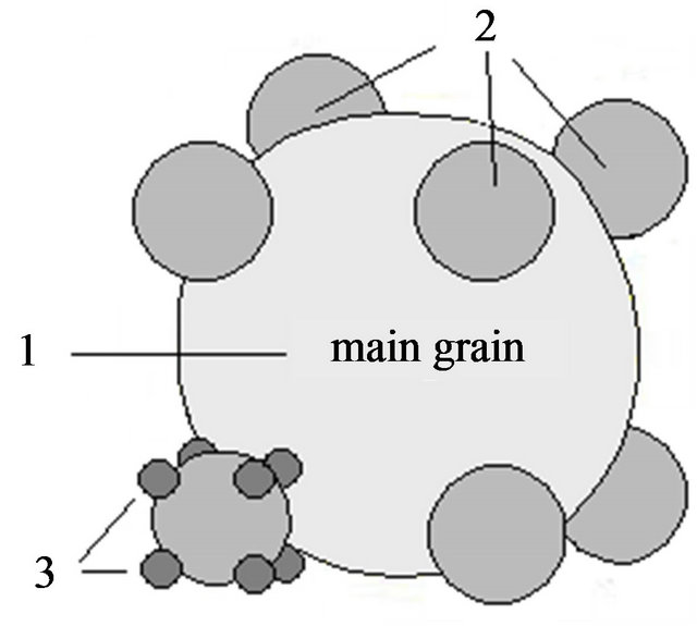 (b)
(b)
Figure 2. Fractal model of clastic sediments.
Table 2. Parameters of fractal model.
However, all spheres are surrounded by planes of double electric layers. The number of fractals composing the solid can be reduced if the size of the first grade becomes smaller. In this case the volume of the double electrical layers will be more considerable. It is easy to calculate the volume of the DEL as the difference between the volume of the solid surrounded by films of adsorbed water and the volume of the pure solid. The thickness of adsorbed water τaw for a salinity of 0.1 mol/l (0.56 g/l) has been accepted as 10−8 m (1e−5 mm) [8]. Obviously the total porosity of the model includes free water, and DEL does not depend on the particle size. However dynamic porosity (the maximal volume of free electrolyte in the pores) depends on the amount of DEL in rocks. Figure 3 demonstrates the influence of DEL on the dynamic porosity of sediments composed by grains of different sizes and number of fractions. Obviously if the sediments are composed of fine grains the number of fractions is limited because the radii of the spheres and the thickness of the DEL are comparable and therefore a considerable part of the pore space is occupied by DEL.
Figure 4 demonstrates the relative amount of DEL in pores for different sizes of first fractals and number of fractals.
The influence of the DEL increases with the amount of clay particles (radius of clay particle is defined as 0.05 mm and less).
2.3. Porosity Parameter
Using (2) and (3) as the equation below describes the porosity parameter PP for a fractal model composed of spheres of different sizes as [6]:
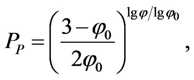 (5)
(5)
where φ0 is an initial porosity, meaning the porosity of the matrix created by the main sediment grains only and φ is the volume of the sediment. Figure 5 demonstrates the dependence of porosity on a models φ0 initial poros-
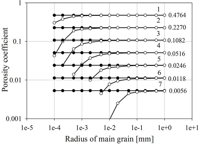
Figure 3. Total and dynamic porosity versus radii of the main grain. Numbers in the figure indicate the number of fractions in the model. Numbers on the right indicate the porosity of the model containing the displayed number of fractions. Closed and open circles indicate the total porosity and dynamic porosity respectively.
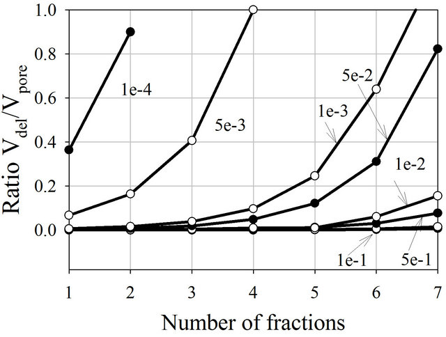
Figure 4. Ratio of volume occupied by DEL to total pore volume Vdel/Vpore depending on the number of fractions making up these diments and the pore radius (in mm).
ity. In the first case PP(φ) is presented as the fractal model. Obviously, with φ0 = 0.4764 as the maximum possible porosity of the matrix represented by a package of identical spheres. For a hexagonal package or a package of identical cubes the initial porosity φ0 will be less. Figure 5 also demonstrates what happens to PP(φ) when φ0 = 0.6. In this case the grains are not packed densely and the mixture is presented as a colloid, however both curves are located very close to each other.
It is therefore possible to use the fractal model to calculate the porosity parameter PP. In the case where the pores have two components (matrix-fluid/gas, non-clay sediments) and the amount of DEL is negligible, the resistivity can be calculated using (2) and (4):
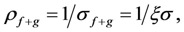 (6)
(6)
where ρf+g is the resistivity of the material filling the pore space (fluid and gas), ξ is the ratio of water occupying the pore spaces of the sediment, and σf is the specific
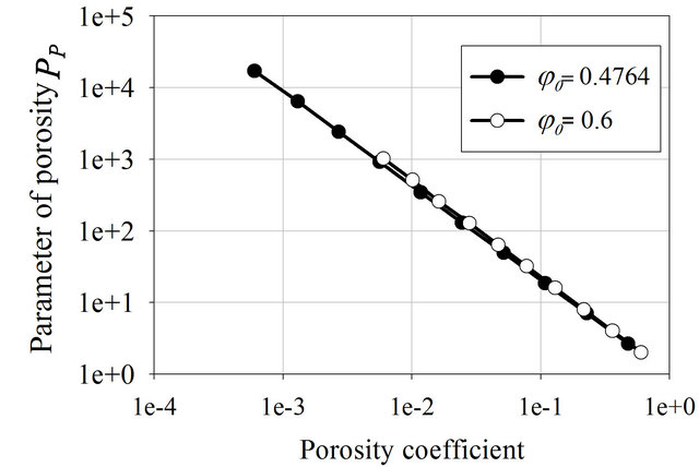
Figure 5. Parameter of porosity PP versus porosity φ for sediments with different initial porosities φ0.
conductivity of the fluid. If the pore space is occupied by a mixture of water, gas and hydrocarbons, the resistivity of the material filling the pore space can be calculated as follows:
 (7)
(7)
where ξ1 and ξ2 are the ratio of water and hydrocarbons occupying the pore spaces of the sediment respectively. However, if the DEL can not be neglected the resistivity of rocks can be calculated using (2), but taking note:
 (8)
(8)
where σfree is the specific conductance of the free solution (or mixture of components filling the pore spaces) and σdel is the specific conductance of DEL.
2.4. Specific Conductivity of the DEL
The specific conductivity of the DEL can be calculated using the Poisson-Boltzman distribution. The density of charges for a symmetrical binary electrolyte is defined by the difference between the concentration of anions and cations [7]:
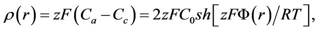 (9)
(9)
where C0 is the salinity of the electrolyte in free solution, Cc and Cc are the salinities of the cations and anions, z is the valence of the ions, and r is the distance from the centre of a pore to its wall. Function Φ(r) is the psi-potential and is described by the Poisson-Boltzman equation. In the inner plane of the DEL Φ(r1) = Φ1, (see Figure 1), where r1 is the coordinate of the outer plane, and the centre of cylindrical coordinates is located in the centre of the pore. Note that the value of Φ1 is very close to the ζ(zeta) potential, and is constant for specific kinds of sediments and must be given a priori. Experiments to measure psi-potentials exist, and the values of Φ2 can be calculated theoretically. Studying ceramic diaphragms, Fridrikh-sberg and Barkovskaya [9] noted that Φ2~170 - 195 mV so we use a value of 180 mV (and consequently Φ1 ≈ ζ ≈ 100 mV). For carboniferous sediments (limestones) numerous experiments showed that ζ~30 - 40 mV and the influence of the DEL will in this case be much smaller.
Numerical integration of the Poisson-Boltzman equation is a very difficult procedure. However as was shown by Kormiltsev [8] there exists an analytical solution: in the case of relatively large pores, Φ(r1) increases very fast with distance from the wall of the solid. Therefore, for large pores the potential distribution in the diffuse part of the DEL can be found using the equation:
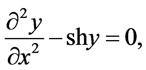 (10)
(10)
where ,
,  ,
,  ,
,  The solution of (10) is:
 (11)
(11)
The average conductance of an electrolyte-filled pore is the ratio of conductivity of a pore to its surface area [8]:
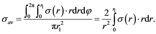 (12)
(12)
Figure 6 demonstrates the average resistivity of an electrolyte (C0 = 0.01 and 0.005 mol/l, ρf = 23.5 and 11.2 Ohmm accordingly), with filled pores of difference size and taking into account the DEL. Porediameters in therange of 1e−4 - 2e−6 mm are common for natural adsorbents such as clays, clayish limestone, a shed tuffs etc. [2]. The influence of the DEL becomes more significant as the pore radius decreases. The conductivity of the DEL can be found using:
 (13)
(13)
The calculated specific resistivity of DEL ρdel = 1/σdel can be accepted as 2.45 - 2.5 Ohmm and 4.90 - 4.95 Ohmm (Figure 7) (for electrolyte salinity C0 = 0.01 and 0.005 mol/l accordingly).
It should be noted that Equation (11) only applies for relatively large pores, however, the resistivity of the DEL of a very thin pore does not differ more than 10% compared to the value obtained for large pores.
2.5. Fractals Containing N-Ellipsoids of Different Size
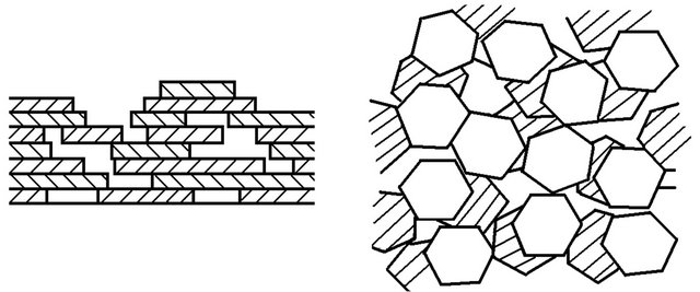
A fractal can be composed not only of spheres but also of ellipsoids, which is important for clays and shields as they are characterized by planar structures (Figure 8).
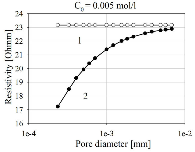
C0 = 0.01 mol/l
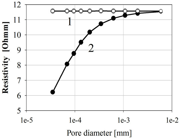
Figure 6. Average resistivity of electrolyte filled pores (water and DEL) versus pore radius.
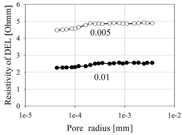
Figure 7. Calculated resistivity of DEL. The curve indices shows the salinity of the electrolyte (C0 = 0.01 mol/l, 0.056 g/l and C0 = 0.005 mol/l, 0.025 g/l).
 (a) (b)
Figure 8. Sediments composed of clays with planar structure, vertical view (a) and top view (b).
In this case the resistivity of packages of identical ellipsoids of rotation can be calculated using the following equation proposed by I. K. Ovichinnikov [2] (Table 1):
 (14)
(14)
where 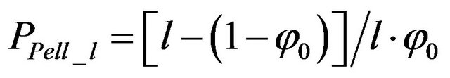 is the parameter of porosity of a model containing oblate ellipsoids of one size, and l is a coefficient of form. Based on previous assumptions, we can construct a fractal model contains n series of rotated ellipsoids of different sizes (Figure 9).
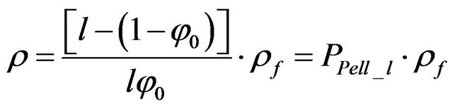
As described above, the first fraction is represented by the biggest grains occupying volume V0, with the rest of the volume φ0 = (1 ‒ V0) occupied by a series of smaller grains. The second fraction of smaller grains will occupy a volume (1 ‒ V0)·V0, etc. The resistivity of the fractal ellipsoid model is then equal to:
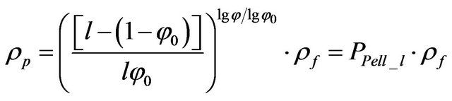 (16)
(16)
where  is the parameter of porosity. Figure 9 illustrates the parameter of porosity PPell_l for different coefficients l. PP for the spherical fractal model is also shown.
In Figure 10, it can be seen that the porosity parameter decreases with increasing oblateness (flattening) of the ellipsoids. The parameter of porosity for the fractal model composed of spheres is also plotted in the figure. This figure shows that the resistivity of sediments depends not only on its porosity and pore sizes, but also on the shape of the sediments. Note that the pore sizes of the ellipsoid fractal model are narrower than the spheroid fractal model, however, the resistivity of sediments with plated structures are lower.
Note that the amount of DELs in the ellipsoid fractal model is higher than in the spheroid fractal model, as one unit of sediments contains considerably more oblate ellipsoids than spheres.
Lithological classification determines the size of clay particles to be approximately 10 µm or less in diameter. Figure 11 demonstrates the relative amount of DEL versus the number of fractions contained in the model for
Figure 9. Fractal model containing n-oblate ellipsoids of different size.
Figure 10. Parameter of porosity for spherical and elliptical fractal models. Indices indicate the coefficient of form l. For spherical particles l = ‒2.
Figure 11. The relative amount of DEL versus the number of fraction containing on the model for different elongated diameter of main ellipse. The curve indices are the coefficients of form l indicating the degree of flattening.
different diameters of the main ellipse of 0.002 mm and 0.02 mm. It can be seen in Figure 10 that the amount of DEL increases considerably as the diameters of the planar clay particles decrease, and decreases with the degree of flattening l. Moreover, if the diameter of plated clay particles is about 0.01 mm or less, the amount of DEL in the pores can dominate over the amount of free water, resulting in the phenomenon of capillary superconductivity. This phenomenon was discovered in Saint Petersburg State University and discussed in [3]. Equation (2) can be presented as:
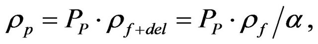 (17)
(17)
where 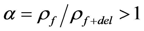 is a coefficient showing the influence of a DEL on the resistivity of the pore space filling. Equation (17) can be written as:
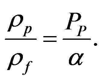 (18)
(18)
The resistivity of sediment ρ increases with increasing PP but decreases with increasing α. For a specific structural construction of grains (planes) making up sediments it can happen that α > PP. Then the resistivity of the sediment becomes lower than when water saturates the pore spaces. The ellipsoid fractal model shows the conditions when α > PP will be satisfied. For example, consider a case where the diameter of clay particles is about 0.002 mm and the sediment contains particles of two sizes. The porosity is equal to 0.227, water salinity is 0.01 mol/l and all pores are filled by DEL with resistivity 2.5 Ohmm (Figures 4 and 11). The calculated resistivity of the clay is  The resistivity of water is 11.6 Ohmm, therefore the resistivity calculated for the clay in this example is lower than the resistivity of free water.
3. Equations for Petrophysical Parameters
3.1. Resistivity of Three Component Sediments
The theoretical value of the resistivity of sediments composed of three components (water, clay and solid matrix) can be calculated using equation [2]:
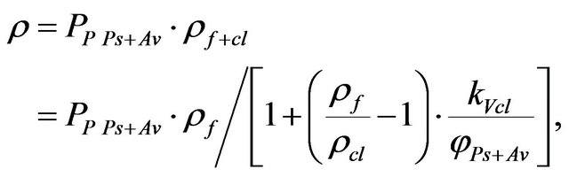 (19)
(19)
where PP Ps+Av is parameter of the porosity of the solid matrix (psammito-aleuritic fraction) (Equation (5)), ρcl is the resistivity of clay, φPs+Av is the porosity of the solid (psammito-aleuritic fraction), kVcl is the volume of the clay in the unit volume of sediments.
The resistivity of clay can be calculated using the following equation:
 (20)
(20)
where, ξ is the volume of pores occupied by free electrolyte, (1 ‒ ξ) is the volume of pores occupied by the DEL (for fractal model see Table 1), and PPcl is the porosity of clay that can be determined using the fractal model.  can be determine using (13).
3.2. Dependence of Permeability on Porosity Using the Fractal Model
The dependence of permeability on porosity for simple matrix models is well known [2]. Referring to our model, the permeability of cubic and rhombic packing of one grain size can be given as:
and
 (21)
(21)
where dk is the diameter of spherical pores, and φ = π/4 for cubic packing and θ = 60˚ for rhombic packing (θ is the angle between the centre of the grains for different levels). Equation (21) demonstrates the dependence of permeability kP on the type of capillary packing, and that the permeability kP is proportional to the pore diameter (to the power of two) and porosity of the model φ.
Let us consider a more complex model, such as a cylindrical sample with a surface area S and length l (Figure 12). This sample can be sheared on n elements with surface areas ωi, and length l. One filtering channel is located inside each unit. The surface area of each filtering channel ωki within the unit is changeable and the length of the filtering channel is equal to lki.
This is a classical Karman-Kozeny model. In this case, the permeability kP of the model is equal to [2]:
 (22)
(22)
where φeff is the coefficient of effective (dynamic) porosity, SFV is the surface of the specific filtering channel in the unit, TH = lk.av/l is the hydraulic tortuosity, f is the Kozeny constant which falls in between 2 and 3 and is usually close to 2.5. The Karman-Kozeny model is regarded as a model closer to real sediments. In this model
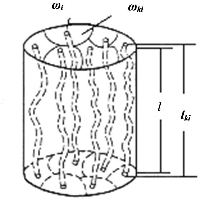
Figure 12. Karman-Kozeny model [6].
the permeability kP is proportional to the cube of the effective (dynamic) porosity φeff, and inversely proportional to the specific surface of a filtering channel and the hydraulic tortuosity, both to the power of two, as well as the Kozeny constant f, which is characterized by the form of the pore channels.
The pore channels are filled with free water and adsorbed water. The DEL occupies a volume φdel, and the thickness of the film of adsorbed water is τav. The final equation for permeability in the Karman-Kozeni model is equal to [2]:
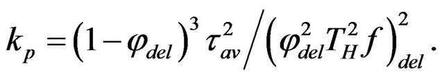 (23)
(23)
Since f ≈ const, TH = const, τav ≈ const for each sediment type, kP depends on φ and φdel. The dependences φ and φdel for a fractal model was shown in Figure 13 (τav = 1e−5 mm). An increasing amount of adsorbed water leads to a decreasing permeability for the sediment. The sediments with permeability less than kP < 0.01 μm2 (<0.01 D) are impermeable. Therefore rocks for which the size of the main grain is less than 1e−5 - 5e−5 m (5 - 10 micron) (clays) are impermeable. However, there is not direct relation between porosity and permeability as the amount of DEL governs the permeability of rocks. Whereas on the other hand, the amount of DEL depends on grain size of rocks.
4. Applications
In 21st century, interpretation of EM data cannot be presented asa comparison of resistivity data any more. There are many publications where the relation between resistivity, porosity, resistivity and permeability has been found statistically. However, even within one type of rocks, the dependence of resistivity on porosity is often different. Moreover the relationship between resistivity and porosity (or permeability) usually is displayed as a

Figure 13. Permeability versus porosity for different amounts of absorbed water.
large cloud of measured values. Statistical method is simply a set of measurements in the laboratory (or boreholes data) without “looking inside pore of pores” and without taking a note of the grain sizes and amount of DEL. A fractal model is a useful tool for the interpretation of electromagnetic data. It can be used to determine porosity, salinity of water, permeability and other electrophysical parameters such as the diffusion coefficient CD and volume of D. Below we shall present some examples of electromagnetic interpretation using the fractal model.
4.1. Search for Fresh Water and an Estimate of the Porosity of Water Bearing Sandstone
Time domain electromagnetic method (TDEM) has been used to search for fresh water in the Orenburg region, Russia. TDEM soundings were located along several profiles. In this area, there are several wells that have been electrically logged. Examples of logging diagrams are shown in Figure 14. Interpretation of TDEM data has been carried out using the software package ERA [10]. This software is a mathematical modelling package and allows for the identification of several layers with different resistivities and thicknesses within a section.
For the calculation of porosity some a prioi parameters have to be taken into account, namely the amount of clay contain kVcl (25%) and salinity of water (0.03 g/l). According to the lithological description, the sandstones contain 25% - 35% clay material. The salinity of the fresh drinking water is recorded as 0.25 - 0.3 g/l. Using these parameters in (19) the porosity of sandstone φPs+Av has been estimated. The PP Ps+Av is parameter of the porosity of the solid matrix and it has been calculated using (5). For calculating theresistivity of clay the fractal
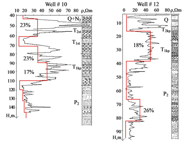
Figure 14. Comparison of TDEM and borehole survey data for aquifers in Orenburg region. Black curve shows the electrical resistivity log, red curves shows the resistivity log from TDEM data. Visual borehole log is shown on the right.
model has also been used. As the porosity of clay is in general approximately 50% and the size of the main grains < 10−8 m [7]. The resistivity of water ρf is equal to:
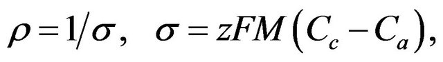 (24)
(24)
where F is the Faraday constant [9.64955·10−4 K/mol], z is the valence, Μ is the mobility of ions (in m2/Vs) and C is the salinity of cations and anions (in mol). Subscripts “a” and “k” indicate anions and cations.
The complete nomogram showing water resistivity’s dependence on salinity and temperature is presented by Itenberg [11]. Calculated resistivity versus porosity coefficients of three component sediments (solid matrix (fractal), clay (fractal) and water) is displayed in the Figure 15. Using this diagram the porosity of the sediments was calculated.
A few layers with different resistivities were identified in the cross-section and a comparison with borehole data and borehole loggings showed good agreement between the logs and TDEM resistivity (Figure 14). The porosity of water bearing sandstones estimated for each layer is 18% - 26% as shown.
4.2. Search for Fresh Water in Permafrost and an Estimate of the Salinity of Water
The TDEM method has been used to define a fresh water aquifer in the polar oil and gas fields of Zapolyarnoe, in the Tumen region, Russia [12]. All TDEM signals were distorted by induced polarization (IP) effect. Mathematical modelling has been used for the interpretation of TDEM data. The home-made software IRAF allowed us to remove the IP effect from the readings, and then the data was interpreted using the standard software ERA [10]. A low resistive layer (6.5 - 8 Ohmm) was observed within the permafrost at a depth of 60 - 70 m. Figure 16 was used to estimate the salinity of the melt water. As the porosity of water bearing sediments can be 20% - 25% and more. therefore, the salinity of water has been calculated

Figure 15. Calculated resistivity versus porosity coefficient of three component sediments. Index of curves is salinity of water (g/l). Volume of clay in unit is 0.25 (25%).
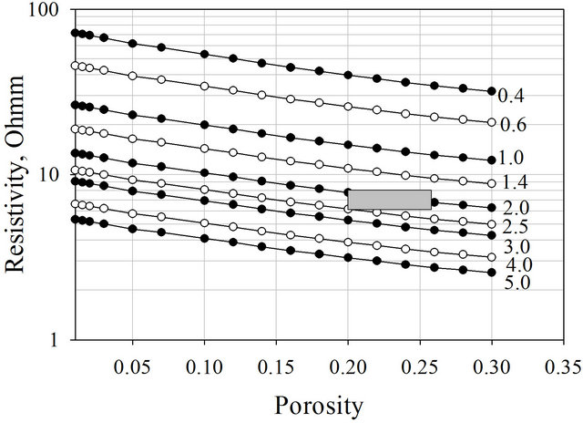
Figure 16. Calculated resistivity versus porosity coefficient forthree component sediments. Indices of the curves show the salinity of the water (g/l). Volume of clay in unit is 0.25 (25%). Square indicates the limit of salinity relative to resistivity 6.5 - 8 Ohmm.
using (19) where the parameter of porosity is presented as fractal. The salinity of water with a resistivity 6.5 - 8 Ohmm was estimated as 2 - 3 g/l (square box in Figure 16). However, well drilling was recommended and completed.
The geological log from a well is summarized below:
0 - 45 dark grey loam, frozen with rare layers of pure ice; 45 - 75 m layering, loam and sandy loam, the sediments are unfrozen within the interval of 62 - 68 m, with a layer of water saturated sand; 75 - 80 m dark grey clay, frozen. With regards to the ground water, the daily pumping rate was 12 - 17 m3/s, and the subsequent chemical analysis resulted in a concentration of 3 g/l. The taste of water is slightly salty, and unfortunately this ground water does not fit the drinking water standard. However, the interpretated TDEM data using (10) and the fractal model show a good agreement with drilling data.
4.3. Estimation of Permeability
Lastly we have selected a number of well characterized sandstone samples for study, although we focus here on measurements made on the Berea, Tennessee, Coconino and Island Rust sandstones. Measurements of samples and analysis have been provided by Baker [13].The mean grain size of each sample has been estimated by Baker using the Havriliak-Negami relationship. Below is a description of each rock unit:
Berea sandstone is of Mississippian age, quarried in Berea, Ohio. The major components of this sandstone are quartz, quartzite lithic fragments and feldspar. The mean grain size of 0.3 mm; the porosity of the Berea sandstone sample is 19%. Coconino is an Early-Permian age sandstone of windblown origin and comes from one of the Grand Canyon formations. The major components of this sandstone are quartz, feldspar, and some lithic fragments. The sandstone porosity is connected with a 0.5 mm mean grainand is equal to 11%. Tennessee Sandstone is of Pennsylvanian age and is part of the Crab Orchard formation. The major components of this sandstone are quartz, feldspar, and some litic fragments. The main grain is 0.2 mm with non-interconnected pore spaces. Porosity is 6%.
Island Rust sandstone is composed mainly of surrounded to angular quartz, with a porosity of 14%. The main grain size is 0.2 mm with pores that are not well connected.
Pore size distribution and permeability of each sample have been measured using the mercury invasion capillary pressure method (MICP), which is the most precise method for study internal structure of rocks. The permeability of the investigated samples measured by MICP are given in the Table 3 (first column) [13].
Another way of predicting permeability was proposed by Berg [14] and presented in [13]. The predicted permeability is presented in the second column.
Zadorozhnaya and Maré [15] proposed a new model of membrane polarization and mathematical consideration. In laboratory, electrical responses for samples with different applied currents were measured and then mathematical modeling of pore structure was carried out. In general for mathematical modeling more than 80 different pore sizes have been used. The number of pores of each size can be varied to achieve a better correlation with measured data. DEL in the walls of the pores has also been considered. The estimated pore permeability for each sample, using (23), is listed in Table 3 (column 3).
The main pore radius has been estimated using both MICP and mathematical modelling. Pore size distribution for Berea, Tennessee and Island samples obtained by MICP and MM are very similar and the main radii of pores are the same for both method. However, we did not obtained a good agreement between MICP and MM for the Coconino sample, therefore an estimation of permeability has been provided for both of these methods. In Table 3 MM data is shown with (*). As we can see the estimated permeability using the fractal model in Table 3 is comparable with the well-known and widely accepted MICP method, Berg’s relationship and the new method
Table 3. Permeability of samples obtained by four different methods.
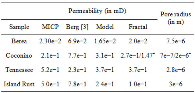
which involves the measurement of samples in the laboratory and mathematical modelling of the pore size distribution.
5. Conclusion
A fractal model containing n-series of spheres with corresponding radii and surrounded by a thin film of adsorbed water tested in this study. This model is more suitable to sedimentary rocks because it not only allows for varying grain sizes and number of fractions, but also takes into consideration the influence of the double electrical layers on the physical properties of sediments. It is also shown that if sediments contain plated particles (for example clay) the resistivity of these sediments can be considerably lower than would be expected, due to a decreasing porosity parameter and more importantly, due to the increasing amount of DEL. Ellipsoid fractal models provided mathematical proof of the phenomenon of supercapillary conductivity observed by laboratory measurements. Using the parameters of the fractal model several petrophysical parameters can be calculated, namely resistivity porosity, and permeability. Mathematical modelling of petrophysical properties can be done to enhance the interpretation of TDEM data. In a case study, layers with different resistivity were identified on a section from a TDEM survey. The results were compared to borehole data and borehole loggings and showed good agreement between the log and TDEM resistivity. In addition, using the given (calculated) resistivity of layers, the porosity and salinity of water bearing layers has been estimated using the fractal model. Estimated permeability calculated using the fractal model showed good agreement with the additional methods (MICP method, Berg’s relationship and mathematical modelling), thus allowing permeability to be determined.
REFERENCES
- G. E. Archie, “The Electrical Resistivity Log as an Aid in Core Analysis Interpretation,” Transactions of AIME, Vol. 146, 1942, pp. 54-62.
- V. N. Kobranova, “Petrophysics, Manual Book,” Nedra, Moscow, 1986.
- O. N. Grigorov, Z. P. Kozmina, A. B. Markovich and D. A. Fridrikhsberg, “Electrokinetic Properties of Capillary Systems,” AN SSSR, Moscow, 1956.
- A. S. Semenov, “Influence of Structure on the Specificresistivity of Aggregates,” Geophysika, Gosgeoltehizdat, Leningrad, Vol. 12, pp. 46-62.
- H. Pape, G. Clauser and J. Iffland, “Variation of Permeability with Porosity in Sandstone Diagnesis Interpreted with Fractal Pore Space Model,” Pure and Applied Geophysics, Vol. 157, No. 4, 2000, pp. 603-619. doi:10.1007/PL00001110
- V. N. Dakhnov, “Interpretation of Results of Geophysical Investigation in Wells,” Gostoptehizdatm, Moscow, 1962.
- D. A. Fridrikhsberg, “Course of Colloid Chemistry,” Khimia, Leningrad, 1974.
- V. V. Kormiltsev, “Electrokinetical Phenomena in Porous Rock,” AN SSSR, Ural Branch, Sverdlovsk, 1995, 47 p.
- D. A. Fridrikhsberg and V. A. Barkovsky, “Study of Surface Conductance, Zeta Potential and Adsorption on Diaphragm of Barium Sulphate,” Kolliodny Journal, Vol. 26, No. 6, 1964, pp. 7-22.
- M. I. Epov, Yu. ADashevsky and I. N. Eltsov, “Automatic Interpretation of Electromagnetic Soundings,” Institute of Geology and Geophysics, Novosibirsk, 1990.
- S. S. Itenberg, “Interpretation of Results of Loggings,” Nedra, Moscow, 1978.
- V. Yu. Zadorozhnaya, “Electroprospecting by TDEM for a Search for Groundwater in Permafrost,” Izv. VUZ, Series, Geologiya i Razvedka, Vol. 3, 1998, pp. 103-106.
- H. A. Baker, “Prediction of Capillary Pressure Curves Using Dielectric Spectra,” Unpublished MSc Thesis, Boston College, Chestnut Hill, 2001.
- R. R. Berg, “Method of Determining Permeability from Reservoir Rock Properties,” Transactions of Gulf Coast Association of Geological Societies, Vol. 20, 1970, pp. 303-317.
- V. Zadorozhnaya and L. P. Maré, “New Model of Polarization of Rocks: Theory and Application,” Acta-Geophysica, Vol. 59, No. 2, 2011, pp. 262-295. doi:10.2478/s11600-010-0041-6