Int'l J. of Communications, Network and System Sciences
Vol. 5 No. 1 (2012) , Article ID: 16688 , 10 pages DOI:10.4236/ijcns.2012.51004
Multi-Resolution Fourier Analysis Part II: Missing Signal Recovery and Observation Results
Faculté des Sciences et Techniques, Université François Rabelais, Parc de Grandmont, Tours, France
Email: nouredine.yahyabey@phys.univ-tours.fr
Received August 27, 2011; revised October 22, 2011; accepted November 4, 2011
Keywords: Fourier Multi-Resolution; Spectral Analysis; Frequency Estimation; Frequency Resolution; Spectral Leakage; Missing Parts; Signal Recovery
ABSTRACT
In this paper, we report application procedures and observed results of multi-resolution Fourier analysis proposed in the first part of this series. Missing signal recovery derived from multi-resolution theory is developed. It is shown that multi-resolution Fourier analysis enhances dramatically performances of Fourier spectra suffering limitations traced to implicit time windowing. Observed frequency resolutions, improvement of frequency estimations, contraction of spectral leakage and recovery of missing parts of finite duration signals are in accordance with theoretical predictions.
1. Introduction
In the first part of this series [1], we proposed multi-resolution Fourier analysis of finite duration signals. We constructed signals from the only observed one able to reveal in the frequency domain resulting transforms whose main lobe-widths between 3-dB levels or resolutions decrease as lengths of constructed signals, called multiresolution signals, increase. Derived expression of multiresolution signals shows that the number of resolution levels are defined by increasing or decreasing the length of multi-resolution signals in order to depict respectively detailed or global views.
In this second part, we report application procedures of multi-resolution signals and missing signal recovery. We propose to observe, via examples, the following performances of multi-resolution theory.
1) The popular FFT algorithm is used for all computations.
2) Frequency axis is magnified or contracted in accordance with applied resolution.
3) Extent of spectral leakage is contracted and improvement of frequency estimation is enhanced in accordance with applied levels of resolution.
4) Inverse transformation recovers missing parts of observed finite duration signals since phase information is not destroyed by multi-resolution signals.
In Section 2, we recall, for easy reference, expression of multi-resolution signals derived from the only observed finite duration signal [1]. Frequency leakage and frequency estimations yielded by multi-resolution signals are reconsidered in Section 3. Expression of recovered missing parts of finite duration signals by means of thresholding in the frequency domain before transforming are detailed in Section 4. Observation results on frequency resolution performances, contraction of leakage, frequency estimation and recovering of missing parts of signals are reported in Section 5.
Observation results show that multi-resolution Fourier analysis enhances dramatically performances of Fourier spectra suffering limitations traced to implicit time windowing [2]. Reported observations are in accordance with theoretical predictions [1].
2. Fundamentals
In this section, we recall for easy reference principal results of [1].
2.1. Definitions
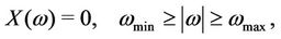
Let  be the bandpass amplitude spectrum of the zero-mean real signal
  defined by,
 (1)
(1)
where  and
and  are the bounds of the spectral support of
 .
.
Let us consider the observation interval whose length T is chosen so that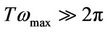 . A finite observation of
  in the time interval of duration T available at the output of a low-pass filter of cut-off frequency
  yields,
 (2)
(2)
The instants , where
  is the sampling frequency, define the discrete-time process
 , rewritten
 .
.
2.2. Expression of Multi-Resolution Signals
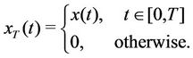
Multi-resolution signals constructed from the only observed finite duration signal  in the time interval of length T are denoted
  where
where  represents the resolution operator of level, s, applied to
 , (see eq. (50) of [1]), i.e.,
 (3)
(3)
where  are resolution levels and I
 is the integer part of
 . Here
  represents the rectangular window of length
 .
.
Angular frequency resolution  of (3) as a function of the level of resolution, s, is given by,
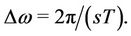 (4)
(4)
3. Frequency Estimation and Spectral Leakage
In the following, frequency estimation and leakage effects are reconsidered for multi-resolution signals.
3.1. Frequency Estimation
It is of an unquestionable interest to detail how precise frequency estimations are provided by multi-resolution signals. Let us assume for the sake of illustration that we have a sinusoidal waveform observed in the time interval of length T whose whose angular frequency is . One can see that lengths of intervals in which a spectral line lies as a function of increasing levels of multi-resolution signals are given by,
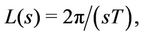 (5)
(5)
where s = 2, 3, 4, 5, represents levels of multi-resolution signals.
This means that the precision with which the angular frequency of the sinusoidal wave is known increases with increasing levels of multi-resolution signals, following in this, decreasing lengths of the interval in which lies .
.
3.2. Spectral Extent of Leakage
To illustrate how frequency extent of leakage is modified when multi-resolution signals are used, let us reconsider here also the sine wave whose angular frequency is . It is well known that the spectrum of a sine wave of angular frequency
  does not consist of one component [3]. A series of magnitudes spaced on the frequency axis with the mutual distance
  tend to display a maximum at the vicinity of
 . This spread of amplitude to adjacent frequency regions, termed leakage [2], depicts a frequency extent given by multiples of
  (see p. 247 of [3]).
In the multi-resolution framework, any angular frequency is given by,
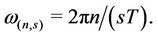
Hence modification of the frequency extent of this series of magnitudes at the vicinity of  as a function of the level of resolution is obtained by considering the variation
 . By using (5), one can see easily that,
 (6)
(6)
where .
.
By increasing the level of resolution, spacing of components on the frequency axis gets smaller and smaller such that angular frequency location of the signal moves closer to its true value. If true frequency location does not meet its integer multiple, then lines gather around its vicinity and the power leaks into much smaller adjacent cells of length . Spectral leakage is therefore contracted in accordance with levels of resolution s where
 .
.
4. Missing Signal Recovery
In this section, we recover missing part of a signal by using multi-resolution signals. We start by reconsidering amplitude spectra of multi-resolution signals in order to recover true spectra by means of filtering.
4.1. Expression of Filtered Spectrum
Fourier transformation of resolved spectral estimates, denoted , is given by (see Equation (44) of [1] for details),
 (7)
(7)
where  is the spectrum of
  depicted with the resolution
  and
and  gathers phases yielded by lengths of local periods of resolution signals.
It is crucial to notice that the spectrum is different from the true spectrum
 . However, the true spectrum can be recovered from (7) as shown below. Accordingto above results on resolution windows, we can write,
 (8)
(8)
By setting (8), (7) yields,
 (9)
(9)
Let us define the action of any filtering operation as an operator F[x] acting on x. An ideal filtering able to recover missing parts of signals by means of inverse Fourier transformationis that filtering able to eliminate the second righthand side of (9) without affecting its first right-hand side.
 (10)
(10)
4.2. Recovering of Missing Parts
According to expression of multi-resolution signals as given by (3), one can see easily that the term  that gathers phases resulting from time translations can be written as,
 (11)
(11)
By using (11) and considering the inverse Fourier transformation, denoted by the operator , of (10) in the window of length sT , represented by
 , we obtain,
 (12)
(12)
which is the recovered signal composed of its original part in the observed interval [0; T] and its missing part in the adjacent interval of length ,where s = 2, 3, 4, 5.
4.3. Type of Filtering
According to above results, one can easily see that (see details in the first part of this series [1]),
 (13)
(13)
Notice also that side-lobes obtained by significant superposition of contributions  and
and 
are observed beyond the interval defined by  [1].
[1].
Here (13) means that we can reduce these side-lobes by applying selected of windows with nonuniform weighting or using one of the threshold selection rules [2]. In this work, for the sake of simplicity and illustration, we propose only hard thresholding procedure justified by(13) and defined by,
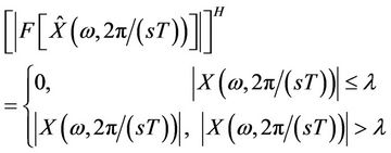 (14)
(14)
where  is the applied threshold value and the upper script H represents hard thresholding. This method sets to zero side-lobes and keeps the spectrum over the threshold.
5. Method and Results
In this section, we report observation results of multiresolution Fourier analysis. Here, the length T of observation intervals is constant and frequency separations  of analyzed signals are so that
 . In order to test resolution capabilities of described multi-resolution signals, let us consider a real signal composed of twoequi-power sinusoids of respective frequencies
  and
and  observed in the constant time interval T and defined by,

In the following subsections we propose to analyze by means of multi-resolution signals these two equi-power sinusoids separated respectively by  and
and  where
where .
.
It is crucial to notice that spectra of multi-resolution signals are represented with their zero-padded versions. We recall that zero-padding resolves all potential ambiguities, smooths the appearance of spectral estimates and reduces the quantization error for the estimation of depicted frequencies [2]. Notice that this zero-padding is a crucial operation since it highlights the effectiveness of the multi-resolution Fourier analysis proposed in the first part of this series and tested here.
5.1. Resolution Schemes and Narrow Bandwidths
Let us choose  Hz and
  Hz satisfying
  where T = 10 s. The instants
 , where
  Hz is the sampling frequencydefine the discrete-time signal
 . The power spectrum of
  is depicted in the plot 1(a1) of Figure 1. Its zero-padded version, as an answer to the question “One or two (spectral lines)?”, is proposed in 1-(a2). As expected, only one powerful spectral line located at 1.1 Hz is depicted.

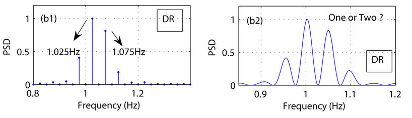
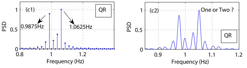
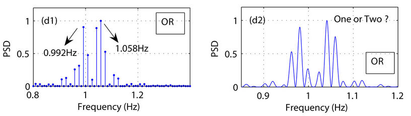
Figure 1. Multi-resolution Fourier analysis of two equi-power sinusoids separated by Δf = 0.5/T. Here (a1), (b1), (c1) and (d1) are respectively double (DR), quadruple (QR) and quintuple (relabeled OR for “optimal”) resolution spectra. Zero-padded versions of (a1), (b1), (c1) and (d1) are shown in (a2), (b2), (c2) and (d2).
5.1.1. Double Resolution Scheme
The power spectrum of the double resolution signal  without filtering is shown in the plot 1-(b1). One can see explicitly two frequencies located respectively at 1.025 Hz and 1.075 Hz. Depicted frequencies correspond respectively to the locations k0 = 41 and k1 = 43 separated by
  for which the double resolution spectrum is zero. In 1-(b2), one finds the zero-padded version of 1-(b1). This shows that we have indeed two separated spectral lines.
5.1.2. Fourfold Resolution Scheme
The power spectrum of the quadruple resolution signal  is shown in 1(c1). We find two sinusoids distributed in the frequency axis defined by quadruple frequency resolution. Depicted frequencies (indicated by arrows) are close to true ones since
  Hz and
  Hz. One notes that the precision with which frequencies are depicted in this scheme are enhanced. The zero-padded version is shown in 1-(c2) where one finds, without ambiguity, two lines separated by
 .
.
It is crucial to notice that the spectrum 1-(c1) (or its zero-padded version 1-(c2)) shows that depicted frequency separations are so that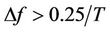 . This means that frequency resolution is indeed effective and it is not destroyed when evolving from a level of resolution to an other one.
5.1.3. Optimal Resolution Scheme
The spectrum of the optimal or the quintuple resolution signal  with its zero-padded version are shown in 1-(d1) and in 1-(d2). Here also, we have an increase of frequency estimations since depicted powerful lines respectively given by
  Hz and
  1.058 Hz are closer to true ones. Here frequency separation between powerful spectral lines is
 .
.
One notes that  is higher than
 . The variation with respect to the true frequency separation,
  , is
, is . This variation meets the corresponding lower bound of the uncertainty principle (
 ).
).
Clearly sinusoids separated by  are well separated by the double, quadruple and optimal resolution signals since depicted frequency separations are greater or equal to lower bounds of their respective uncertainty principles (
 ,
, ,
, ).
).
5.2. Frequency Resolution Limits
Now frequencies are so that  with
with 
 Hz and
  Hz. This frequency separation represents the limit of resolution schemes. Results are shown in Figure 2.
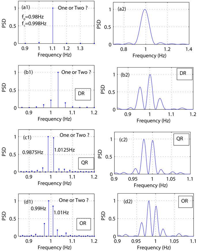
Figure 2. Multi-resolution Fourier analysis of two equi-power sinusoids separated by Δf = 0.18/T. Here (a1), (b1), (c1) and (d1) are respectively double (DR), quadruple (QR) and quintuple (relabeled OR for “optimal”) resolution spectra. Zero-padded versions of (a1), (b1), (c1) and (d1) are shown in (a2), (b2), (c2) and (d2).
One finds in 2-(a1) or 2-(a2), respectively, the spectrum of  and its zero-padded version. This spectrum cannot exhibit the true frequency resolution whatever applied zero-padding. The spectrum of
  in 2-(b1) shows only one powerful frequency located at 1.025 Hz. Its zero-padded version in 2-(b2) depicts however two powerful peaks since zero-padding eliminates potential ambiguities and reduces quantization error.
5.2.1. Fourfold Resolution Scheme
The spectrum of  in 2-(c1) and its zeropadded version in 2-(c2) depict two powerful frequency lines (shown by arrows) located respectively at
0.9874 Hz and  = 1.0125 Hz. These lines are separated by
  which yields a variation of
  with respect to the true frequency separation. It can thus be seen that fourfold frequency resolution scheme is able to separate lines closer to its resolution capability
 .
.
5.2.2. Optimal Resolution Scheme
One can see in 2-(d1) and in 2-(d2), shapes of the two
sinusoids (separated by  in the quadruple resolution scheme) in the new frequency axis defined by optimal frequency resolution
 . We obtain two equipower lines located respectively at 0.99 Hz and 1.01 Hz which yields a frequency separation closer to the true one.
One can see without ambiguity that observed frequency resolutions of Figures 1 and 2 are not limited by the length of the time interval and meet bounds of the uncertainty principle. Results of Figures 1 and 2 show that zero-padding highlights the effectiveness of the multiresolution Fourier analysis. Hence, observed frequency resolution capability of multi-resolution signals is in accordance with theoretical predictions.
5.3. Missing Signal Recovery
Here we consider a signal composed of two sinusoids of respective frequencies  Hz and
  Hz observed in the time interval of length
  s. These frequencies are separated by
 . The original signal,
  , is shown in Figure 3(a) where the missing part is represented by zeros in the interval
 . The spec-

Figure 3. Missing signal recovery. Missing part in the time domain is recovered in (d) by inverse Fourier transformation applied to the thresholded double resolution spectrum in (c).
trum of the double resolution signal  is depicted in Figure 3(b) around the Fourier frequency 1 Hz. One finds two lines at
  Hz and
  1.075 Hz. As already mentioned in section IV, recovering missing part of the signal requires thresholding of the obtained amplitude spectrum in 3-(b). One can see that side-lobes in 3-(b) around powerful spectral lines can be eliminated by applying one of the threshold selection rules as detailed in section IV. In this work, we use hard thresholding procedure with a threshold, as given by (14), is
 . The resulted spectrum is shown in Figure 3(c) where side-lobes are eliminated. Inverse Fourier transformation is applied to the thresholded amplitude spectrum shown in 3-(c). The obtained signal in the interval
  is depicted in 3-(d). One can see that missing part of the original signal composed of two frequencies is indeed recovered.
5.4. Frequency Estimation
Here we use the amplitude spectrum of 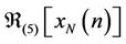 for direct estimation of frequencies. Let us consider the signal
  consisting of sinusoids whose true frequencies are:
  Hz,
Hz,  Hz and f2 = 7.385 Hz observed in the time interval of length
  s. Results are shown in Figure 4. In the plot 4(a), the amplitude spectrum of
  whose frequency locations are separated by the mutual distance
  Hz depicts the frequencies (shown by arrows):
  Hz,
Hz,  Hz and
  Hz. Errors affecting these frequencies are respectively 4.5%, 3% and 1.5%. Clearly, the resolution
  is not able to recover true frequency precisions.
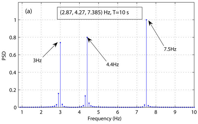
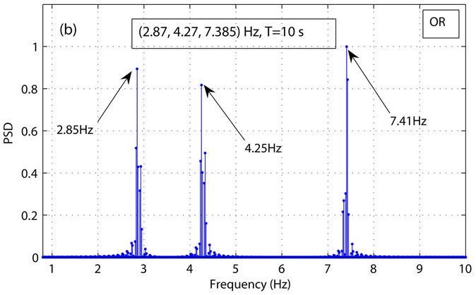
Figure 4. Frequency estimations. True frequencies are: f0 = 2.87 Hz, f1 = 4.27Hz and f2 = 7.385 Hz. Quintuple (or Optimal) resolution Fourier analysis yields frequency estimations in (b) whereas in (a) frequencies are depicted with the resolution 1/T. Estimation Errors in (b) for f0, f1, f2 are respectively: 0.7%, 0.5% and 0.3%.
Now, let us consider the amplitude spectrum of  , (Optimal resolution signal) shown in 4-(b). This spectrum whose frequency locations are separated by the mutual distance
  Hz depicts the following frequencies (shown by arrows):
  Hz,
Hz,  Hz and
  Hz. One can see that frequencies shown by arrows move closer to true ones and are within the resolution
 . Errors affecting frequency estimations are respectively: 0.7%, 0.5% and 0.3%. Frequency precisions are respectively enhanced by 5, 6.43 and 6 with respect to those depicted in 4-(a) by the spectrum of
 .
.
5.5. Extent of Spectral Leakage
Here, we explore the shape yielded by the spectrum of one sinusoid observed in an interval of length T as a function of the level of multi-resolution signal. We propose to observe the frequency extent of the spectrum of a sinusoid as an indication of leakage affecting its spectral line.
Let us consider a sinusoid whose frequency is f = 1.05 Hz observed in the time interval  s. Obtained results are shown in Figure 5. One finds the spectrum of
  in 5-(a), its double, fourfold and optimal resolution spectra are respectively shown in 5-(b), 5-(c) and 5(d). Dotted curves in 5-(b), 5-(c) and 5-(d) represent the spectrum of 5-(a) for comparison.
Let  denote the original extent of leakage of the spectrum 5-(a). The double resolution spectrum 5-(b) exhibits one powerful frequency line located at 1.075 Hz with two side-lobes. Here the variation from one sidelobe to the other one in the interval [1,1.25] (Hz) is
  where the lower script “(2)” stands for “double resolution”. One notes that the extent in which frequency lines are confined is contracted since
 .
.
The quadruple resolution spectrum 5-(c) shows two powerful lines located respectively at 1.0375 Hz and 1.0625 Hz. Notice that the frequency 1.05 Hz coincide with the frequency location for which the quadruple resolution spectrum is zero. This gives two lines instead of a simple one. Variation from one line to the other one is . The extent of the depicted sinusoidal spectrum is
 .
.
In 5-(d), the spectrum of  yields one powerful frequency line located at 1.05 Hz (which is the true frequency). Total variation when including sidelobes (situated in the interval [1.02,1.08] (Hz)) is
 . In 5-(d) leakage is contracted by the factor 5. One notes that components of the spectrum in 5-(d) are spaced by the mutual distance
  which is the fifth part of the distance
  separating components in 5-(a).

Figure 5. Leakage effects. Frequency extent of spectral leakage is reduced as level of resolution increases. Dotted curves in (b), (c) and (d) represent the spectrum (a) for comparison. DR, QR and OR stand respectively for double, quadruple and quintuple (optimal) resolution.
It can thus be seen easily that extent of spectral leakage is successively contracted and observed lines move towards the true frequency in accordance with applied resolution levels.
6. Conclusion
In the second part of this series, we report application procedures of multi-resolution Fourier analysis proposed in the first part of this series together with missing signal recovery. We have shown that frequency resolution of finite duration signals is increased, extent of their spectral leakage contracted, their frequency estimation improved and missing parts recovered without further observation. Performances of Fourier spectra are enhanced in accordance with applied resolution levels. Obtained frequency resolutions are not limited by the length of the observation interval and meet bounds of the indeterminacy principle or Heisenberg inequality. Observed results are in accordance with theoretical predictions.
REFERENCES
- N. Yahya Bey, “Multi-Resolution Fourier Analysis Part I: Fundamentals,” International Journal of Communications, Network and System Sciences, Vol. 4, No. 6, 2011, pp. 364-371. doi:10.4236/ijcns.2011.46042
- S. M. Kay and S. L. Marple, “Spectrum Analysis-A Modern Perspective,” Proceedings of the IEEE, Vol. 69, No. 11, 1981. doi:10.1109/PROC.1981.12184
- E. Terhardt, “Fourier Transformation of Time Signals: Conceptual Revision,” Acustica, Vol. 57, 1985, pp. 242- 256.
- D. L. Donoho and P. H. Stark, “Uncertainty Principles and Signal Recovery,” SIAM Journal on Applied Mathematics, Vol. 49, No. 3, 1989, pp. 906-931. doi:10.1137/0149053