Journal of Intelligent Learning Systems and Applications
Vol. 5 No. 1 (2013) , Article ID: 27937 , 10 pages DOI:10.4236/jilsa.2013.51004
Training with Input Selection and Testing (TWIST) Algorithm: A Significant Advance in Pattern Recognition Performance of Machine Learning
![]()
1Semeion Research Center of Sciences of Communication, Rome, Italy; 2Department of Mathematical and Statistical Sciences, University of Colorado, Denver, USA.
Email: *m.buscema@semeion.it
Received September 30th, 2012; revised November 23rd, 2012; accepted November 30th, 2012
Keywords: Neural Networks; Machine Learning; Pattern Recognition; Evolutionary Computation
ABSTRACT
This article shows the efficacy of TWIST, a methodology for the design of training and testing data subsets extracted from given dataset associated with a problem to be solved via ANNs. The methodology we present is embedded in algorithms and actualized in computer software. Our methodology as implemented in software is compared to the current standard methods of random cross validation: 10-Fold CV, random split into two subsets and the more advanced T&T. For each strategy, 13 learning machines, representing different families of the main algorithms, have been trained and tested. All algorithms were implemented using the well-known WEKA software package. On one hand a falsification test with randomly distributed dependent variable has been used to show how T&T and TWIST behaves as the other two strategies: when there is no information available on the datasets they are equivalent. On the other hand, using the real Statlog (Heart) dataset, a strong difference in accuracy is experimentally proved. Our results show that TWIST is superior to current methods. Pairs of subsets with similar probability density functions are generated, without coding noise, according to an optimal strategy that extracts the most useful information for pattern classification.
1. Introduction
Validation protocol and input selection are some of the most relevant problems in pattern recognition for machine learning. The two most important problems are:
a) how to generate an optimal pair of training and testing set statistically representative of the assigned problem;
b) how to select the minimum number of input features able to maximize the accuracy of the dependent variables (target) in a blind test.
We will show that the TWIST algorithm (Training with Input Selection and Testing) is not only a useful scientific way to approach these two problems but is superior. Therefore this article is going to present:
1) the TWIST methodology;
2) standard methods;
3) how we test TWIST: a) by showing it is not noise; b) use it on a medical problem that has been solved via different machine learning algorithms;
4) report on the results followed by a discussion.
2. Validation Protocol
The issue of the Validation Protocol (VP) is well known in machine learning literature. We can distinguish different types of procedures: K Fold Cross Validation, Leave One Out (a limit case of the first one), Boosting, 5 × 2 Cross Validation, Training set and Testing set splitting, and others [1]. In any case, all these procedures represent different statistical strategies to generate tasks for machine learning training and testing. But any single distribution of the source dataset in a training set and in a testing and/or a validation set is always processed by a random splitting that record (observation) of the source dataset. The reason for the random criterion is a statistical one. Because the source dataset represents all the knowledge that we have of an assigned problem, we need to generate two subsets of data more or less equivalent each other, from a statistical point of view. Consequently, if this is true, the training session will represent a good learning set for the learning machine and the results of testing session will be representative of the machine learning capability to generalize for the whole dataset. We maintain that this is a valid and necessary criterionbut it is not the only one. A second criterion that we feel is necessary is that for a given analysis we are performing on the dataset, each record should contain only those variables that affect the analysis.
The usual approach is a single criterion, the random criterion that aims to optimize the following cost function:
 (1)
(1)
where:
 and
and 
are equal to the probability density function of testing and training subset, respectively, and
is equal to the probability density function of the global dataset.
This means that the random criterion aims to generate two subsets with, more or less, the same probability density function, and, additionally, each one of these subsets should be statistically equivalent to the global dataset.
The random criterion tries to attain the optimal cost function value as defined by Equation (1). But to optimize this cost function we should consider every possible combination of each record split into the two subsets and then for any combination to measure and to compare the probability density function of each subset. There is no evidence that the random criterion can optimize this cost function. Moreover, there are on the order of N factorial possible ways to divide up a database of N records which for a database with 100 records is already prohibitive. However, constraints are imposed which brings the complexity down but nevertheless, it is very hard to compute the global optimum of Equation (1).
Now, given a dataset DG of N records, the number of possible samples dG of k records is given by:
 . Varying k, you have:
 , (2)
, (2)
But the effective space of solutions is smaller, because we have to consider two different constraints:
a) the training and the testing subsets distribution is symmetrical (AB = BA);
b) the number of records in both subsets can be no fewer than the number of the classes (C) of a task (for example, a pattern recognition or a classification task).
Consequently, the effective space of the solutions of the binomial permutation becomes:
 (3)
(3)
where:
N = Number of Records;
 = Number of effective Training-Testing distributions;
k = Number of records in Training or Testing sub sets;
C = Number of the Classes for the pattern recognition.
For example, let us compute the number of splits for a dataset of 10 records (N = 10) where we have two classes (C = 2) in a pattern recognition analysis. In this case the global space of the solutions is 210, while the space of the acceptable solutions is
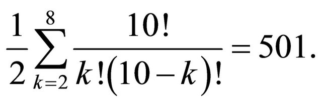
Table 1 and Figure 1 relate the details of this example.
The difference between the global space and the effective space of possible splitting of an assigned dataset is fundamental in pattern recognition analysis. This is because any machine learning needs to have the number of records, both in Training set and in Testing set, equal or bigger than the number of the classes to be learned and validated.
Let us compute again, the number of splits given a dataset of only 4 records and 2 classes: Dataset = {a,b,c,d}, where {} is the set of the records. In this case, the number of all solutions is 24 (that is 16). Applying Equation (2), the number of effective solutions is 6, but applying Equation (3), the number of effective solutions is only 3.
Table 2 shows some details of the global binomial distribution while Table 3 shows the effective number of possible solutions.
Table 1. Global and acceptable (in grey) number of solutions with 10 records and 2 classes.
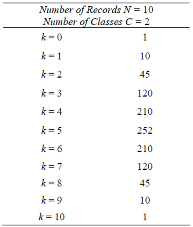
Table 2. Binomial distribution of 4 records.

Table 3. Binomial effective number of possible splitting.
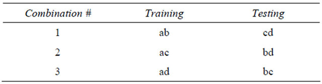
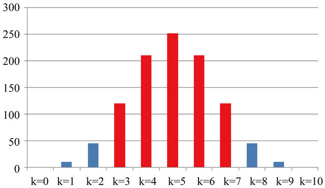
Figure 1. Graphic distribution of global and acceptable (in red) number of solutions with 10 records and 2 classes.
Therefore, a pair of training and testing sets represents, on the solutions space, a possible solution
given by the vector:
 (4)
(4)
where
represents the space of possible solutions for any Training and Testing splitting.
The problem described by Equations (1)-(4) is a typical problem of operation research. For this type of problem, to optimize the cost function (1), we propose an evolutionary algorithm whose population expresses, after each generation, different hypotheses about the splitting of the global dataset into two subsets. To be specific, at any generation each individual of the genetic population indicates which records of the global dataset have to be clustered into the subset A and which one into the subset B. From a technical point of view this is very easy. Each individual of the genetic population is a vector of N Boolean values (1 or 0), where N is the number of the records of the global dataset. From a practical or operational point of view, genetic algorithms are able to effectively deal with problems of high (impossible) complexity such as the complexity of the problem of splitting a database into two sub-databases.
The main problem at this point is to define a suitable fitness function able to adequately evaluate which of the ways of splitting a dataset in two is best. In other words: which of the splitting generates two subsets whose probability density functions are most similar?
To optimize these constraints we have used two independent Supervised Neural Networks (SNNs). Typically we use a Multilayer Perceptron (Back Propagation based). The fitness evaluation of each splitting works in five independent steps, each time that each individual of the genetic population presents its hypothesis of splitting the global dataset into two subsets, subset A and subset B:
1) the first SNN (SNN_A) is initialized and trained using the subset A, and it is stopped when the training error, as the Root Medium Square Error (RMSE), is minimized;
2) the SNN_A, with the trained weights fixed, is applied in a blind way on the subset B, and its accuracy is saved;
3) the SNN_B, completely independent from the SNN_A, is initialized and trained using the subset B, and it is stopped when the training error (that is, for example, the RMSE) is minimized;
4) the SNN_B, with the trained weights fixed, is applied in a blind way on the subset A, and its accuracy is saved;
5) the minimum value of the two accuracies is assigned as fitness of the hypothesis of splitting, generated by any individual of the genetic population.
The steps from 1 to 5, called “Fitness Evaluation” are executed for each individual of the genetic population, at any generation of the evolutionary algorithm.
The flow chart of the whole algorithm is as follows:
a) Genetic Population Initialization b) Evolutionary Loop i) Fitness Evaluation of the proposal of splitting of each individual of the genetic population at the generation (n) (From step 1 to step 5);
ii) Crossover and offspring are produced;
iii) Random mutation is applied;
iv) Setup of the new population;
v) If the average fitness continues to grow start from the beginning; else terminate;
c) Save the subset A and the subset B with the best fitness.
This algorithm is named Training & Testing Optimization (for short T&T). The advantages of T&T algorithm are many:
1) The evolutionary loop uses a special enhancement of the classic genetic algorithm. Its name is Genetic Doping Algorithm (for short GenD). GenD has shown to be more effective than the classic genetic algorithm in many optimization problems [2];
2) The Multilayer Back Propagation, using the SoftMax algorithm [3] for classification tasks, is a very robust and fast ANN (for the most of the classification problems 100 or 200 training epochs are enough). Furthermore, Back Propagation SNN is also able, with an suitable number of hidden units, to compute any continuous function [4,5];
3) The reverse procedure of T&T algorithm (steps 3 and 4 are the reverse of steps 1 and 2), the kernel of the algorithm, finds two subsets whose density probability functions are pretty similar. This is not an advantage, but it is a right prerequisite for pessimistic training and testing distribution.
4) The T&T algorithm is a powerful tool that uses all the information present in the global dataset. Moreover, the optimized Subset A and Subset B can be used both for Training and Testing (learning from subset A and evaluate using subset B, and vice versa), with different learning machines (Neural Networks, Decision Trees, Bayesian Networks, etc.). Our comparison with the classic random criterion to setup the Training and the Testing set shows that the T&T algorithm significantly outperforms random distribution strategy on real medical applications [6-18].
3. Input Selection
Another significant methodological problem related to the application of Machine Learning to real databases becomes apparent when datasets are comprised of a large number of variables which, apparently, seem to provide the largest possible amount of information. When we use these large databases in, for example, classification tasks, the input space, determined by all the possible combinations of the values of the observed variables, becomes so large that any research strategy to find the best space for the task becomes very cumbersome in some cases and impossible in others.
It is necessary to carry out a preliminary analysis of the variables of the dataset since these can have a different relevance with respect to the data mining that one intends to carry out. Some of the attributes may contain redundant information which is included in other variables or include inconsistent information (noise) or may not even contain any significant information at all and be completely irrelevant. Therefore a procedure that will identify and select, from the global set, a subset consisting of those variables that are most informative in the representation of input patterns is necessary when dealing with classification problems solved with induction algorithms. Moreover, the accuracy of the procedure, learning time and the number of examples necessary are all dependent upon the choice of variables.
Among the methods used to reduce the dimensionality of the data, the Feature Selection techniques (also known as Subset Attribute Selection or Input Selection) were developed to determine which variables (or attributes) are most relevant in the representation of an input pattern, starting from a large dataset [19-29].
When dealing with a database with a large number of variables, we use Feature Selection to try to reduce the number of variables that are used in the classification while maintaining an acceptable level of accuracy in the procedure. By extracting the most relevant attributes, the dimensions of the input space is reduced. Thus, when we only use the most relevant attributes, it is easier to find the best solutions and, if the extracted attributes are actually the most significant, the predictive capability in the global data is most effective.
On the whole, Feature Selection extracts from a given dataset DG of M characteristics the best subset consisting of K characteristics. The number of possible subsets of K characteristics is given by:
and between these the best one is the one that maximizes the generalization of the machine learning in the test phase.
Excluding the exhaustive search strategy on the global set of characteristics, which is not applicable to a dataset with a high number of variables, the techniques that can be used are a blind search (for example, Depth First) or heuristic (Hill Climbing, Best First). In the literature, evolutionary search techniques have also been proposed [24,30,31].
Feature Selection techniques can be developed using two different general approaches based on whether the selection of the variables is carried out dependently or independently of the learning algorithm used to build the inductor. The filter approach attempts to select the best attribute subset by evaluating its relevance based on the data. The “wrapper” approach, instead, requires that the selection of the best attribute subset takes place considering as relevant those attributes that allow the induction algorithm to generate a more accurate performance [32].
Our Input Selection algorithm (IS) operates as a specific evolutionary wrapper system that responds to the need to reduce the dimensionality of the data by extracting the minimum number of variables necessary to conserve the most information available.
Thus, to integrate our IS algorithm with T&T algorithm into one procedure we have to modify the structure of each individual of the genetic population, which has already been described.
This fusion of IS with T&T is a complex algorithm able to look for the best distribution of the global database divided in two optimally balanced subsets containing a minimum number of input features useful for optimal pattern recognition. We have named this new algorithm TWIST (Training with Input Selection and Testing).
This integration is as follows. In the T&T algorithm each individual of the genetic population is a vector of N components with Boolean values, where N is the number of the records of the global dataset. When the value of a generic component of the vector is 1, then that record is saved into the subset A, and when the value is 0, then the record is saved into the subset B.
In the IS algorithm, on the other hand, each individual of the genetic population has to be a vector of M components with Boolean values, where M is the number of all the input variables of the global dataset. In this case, when the value of a generic component of the vector is 1 the corresponding input feature is saved into the subset A and the subset B, while if the value is 0, then the corresponding input feature is removed.
Consequently, in the TWIST algorithm every individual of the genetic population will be defined by two vectors of different lengths:
1) the first one, showing which records (N) have to be stored into the subset A and which ones have to be stored into the subset B;
2) the second one, showing which inputs (M) have to be used into the two subsets and which one have to be deleted.
After this modification the TWIST algorithm works as well as the T&T algorithm, already described. At the end of its evolution TWIST will generate two subsets of data with a very similar probability density of distribution and with the minimal number of effective variables for pattern recognition.
Figure 2 depicts the dynamic of the TWIST algorithm.
4. Falsification Test
We show here that the application of T&T and of TWIST algorithms outperforms the other splitting strategy (i.e. random distribution) in terms of results when they are applied to real medical data and also to classic datasets available from the UCI Machine Learning Repository [33].
The “reverse strategy” used in these algorithms tends to generate two subsets with the same probability density function, and this is exactly the gold standard of every random distribution criterion [1]. In addition, when the “reverse strategy” is applied, two fitness indicators are generated: the accuracy on the subset B after the training on the subset A, and the accuracy on the subset A after the training on the subset B. But only the lower accuracy of the two is saved as the best fitness of each individual

Figure 2. Flow chart of TWIST algorithm.
of the genetic population rather than an average of the two or the highest of the two and thus we are conservative. Moreover, this criterion increases the statistical probability that the two sub-samples are equally balanced during the genetic evolution because of the quasi logarithmic increase of the optimization process.
In any case we can apply to the same dataset the TWIST and T&T algorithms many times and we analyze our results using a 5 × 2 Cross Validation protocol (DIETTERICH 1998). To further insure the validity of our approach, we have submitted T&T and TWIST to a falsification test. If we generate a random dataset with a dependent variable randomly distributed we have two possible outcomes:
1) a set of learning machines using the subsets and the inputs selected by T&T and TWIST show better results than the same learning machines trained and tested using sub-samples generated by means of a random splitting and K-Fold cross validation;
2) the set of learning machines using the subsets and the inputs selected by T&T and TWIST show the same results than the same learning machines trained and tested using sub samples generated by means of a random splitting and K-Fold cross validation.
Only if outcome 2 is true does TWIST and T&T behave as a random strategy when there is no information available in the dataset, and consequently validate their capability to extract useful information in datasets, when this information is really present.
To test this hypothesis we have generated a dataset of 1000 records, each one composed of 20 random input variables and one random label as dependent variable. Then we have processed the dataset using 4 different strategies:
1) a K-Fold cross validation (K = 10);
2) a random splitting of the dataset into two subsets, to be used both as training set and testing set;
3) the T&T strategy to generate two subsets to be used both as training set and testing set. T&T algorithm was implemented using a population of 500 individuals and each Back Propagation algorithm was trained for 200 epochs. T&T was run for 1000 generations.
4) the TWIST strategy was implemented to generate two new subsets with a minimal number of variables to be used both as training set and testing set. The TWIST algorithm was also programmed with a population of 500 individuals and the two Back Propagation runs of each individual was trained for 200 epochs. TWIST after the 1000 generations selected 9 input variables from the original 20.
Then we have processed the dataset using 4 different strategies:
1) a K-Fold cross validation (K = 10);
2) a random splitting of the dataset into two subsets, to be used both as training set and testing set;
3) the T&T strategy to generate two subsets to be used both as training set and testing set. T&T algorithm was implemented using a population of 500 individuals and each Back Propagation algorithm was trained for 200 epochs. T&T was run for 1000 generations.
4) the TWIST strategy was implemented to generate two new subsets with a minimal number of variables to be used both as training set and testing set. The TWIST algorithm was also programmed with a population of 500 individuals and the two Back Propagation runs of each individual was trained for 200 epochs. TWIST after the 1000 generations selected 9 input variables from the original 20.
We have used 13 different learning machines, representing the different “families” of the main algorithms known in literature. For each one of the four strategies, the 13 algorithms were implemented using the wellknown WEKA software package [34]. These are the list of the machines learning algorithms used in this comparison [35-38]:
a) Bayes Net;
b) Naïve Bayes;
c) Support Vector Machine (SVM);
d) Logistic Regression;
e) Multilayer Perceptron;
f) Sequential Minimal Organization (SMO);
g) IBk;
h) K Star;
i) Ada-Boost M1;
j) Logit Boost;
k) RotationForest;
l) J48;
m) Random Forest.
The comparison shows clearly that outcome 2 is true (see Table 4), when there is no information in the dataset, the behaviors of the four validation strategies are absolutely equivalent. Therefore, T&T and TWIST do not code noise to reach optimistic results.
5. A Test from Medical Data
Now we will compare T&T and TWIST algorithms with K-Fold CV and Random Training and Testing, using a known medical dataset: Statlog_Heart [39]. The dataset is composed of 13 attributes, two classes and 270 records. TWIST was set with a population of 200 individuals and each ANN (a Back Propagation) was set up with 500 epochs, 12 Hidden units and a fixed learning coefficient of 0.1. After 266 generations the algorithm did not increase its performance.
Attribute Information:
Table 4. Falsification test—results of the comparison.

1) age 2) sex 3) chest pain type (4 values)
4) resting blood pressure 5) serum cholesterol in mg/dl 6) fasting blood sugar > 120 mg/dl 7) resting electrocardiographic results (values 0, 1, 2)
8) maximum heart rate achieved 9) exercise induced angina 10) old peak = ST depression induced by exercise relative to rest 11) the slope of the peak exercise ST segment 12) number of major vessels (0 - 3) colored by fluoroscopy 13) thal: 3 = normal; 6 = fixed defect; 7 = reversible defect.
Variable to be predicted:
Absence (1) or presence (2) of heart disease (we have not considered a specific cost matrix for this application).
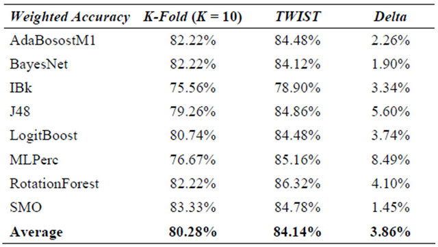
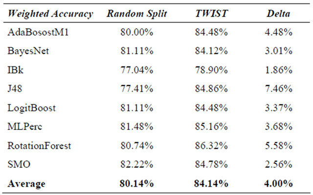
For this comparison we have used only the 8 learning machines that had the best performances in K-Fold CV from among the 13 algorithms considered in the falsification test.
In Table 5 the results are compared. It is evident that machine learning increases their performance when T&T and/or TWIST are used. It is evident in the same way that not every type of machine learning benefits to the same degree from the T&T and TWIST algorithms. Multilayer Perceptron has the best results in each comparison for the simple reason that it is the same machine learning used for T&T and TWIST optimization. But also decision Tree base machines with TWIST and T&T outperform their previous results.
What is really surprising is that many decision Trees and sometime also probabilistic networks increase dramatically their results using this new validation strategy.
Also, TWIST attains the best results by reducing from 13 to 5 the number of attributes.
TWIST selected attributes:
1) age 3) chest pain type (4 values)
9) exercise induced angina 12) number of major vessels (0 - 3) colored by fluoroscopy 13) thal: 3 = normal; 6 = fixed defect; 7 = reversible defect.
6. Conclusions
The results presented here indicate that the T&T and TWIST algorithms:
a) do not code noise to reach optimistic results;
b) are suitable algorithms to generate pairs of subsets with similar probability density function;
c) are optimal strategies that allow machine learning to extract from a dataset the most useful information for pattern classification.
The potential downside of this approach is the CPU time when the datasets are huge. To avoid this problem, we are planning the parallelization of the genetic evolu
Table 5. Statlog heart dataset—results of t&t, twist, k-fold cv and random splitting.
(a)

(b)
(c)

(d)
tion of T&T and of TWIST.
An optimal parallelization and a more intensive experimentation with large datasets will show how much these two new strategies are promising from practical application.
REFERENCES
- T. G. Dietterich, “Approximate Statistical Tests for Comparing Supervised Classification Learning Algorithms,” Neural Computation, Vol. 10, No. 7, 1998, pp. 1885-1924. doi:10.1162/089976698300017197
- M. Buscema, “Genetic Doping Algorithm (GenD): Theory and Application,” Expert Systems, Vol. 21, No. 2, 2004, pp. 63-79.
- J. S. Bridle, “Probabilistic Interpretation of Feedforward Classification Network Outputs, with Relationships to Statistical Pattern Recognition,” In: F. Fogelman-Soulié and J. Hérault, Eds., Neuro-Computing: Algorithms, Architectures, Springer-Verlag, New York, 1989.
- Y. Chauvin and D. E. Rumelhart, “Backpropagation: Theory, Architectures, and Applications,” Lawrence Erlbaum Associates, Inc. Publishers, Hillsdale, 1995.
- D. E. Rumelhart, G. E. Hinton and R. J. Williams, “Learning Internal Representations by Error Propagation,” In: D. E. Rumelhart and J. L. McClelland, Eds., Parallel Distributed Processing, Vol. 1 Foundations, Explorations in the Microstructure of Cognition, The MIT Press, Cambridge, 1986.
- M. Buscema., E. Grossi, M. Intraligi, N. Garbagna, A. Andriulli and M. Breda, “An Optimized Experimental Protocol Based on Neuro-Evolutionary Algorithms. Application to the Classification of Dyspeptic Patients and to the Prediction of the Effectiveness of Their Treatment,” Artificial Intelligence in Medicine, Vol. 34, No. 3, 2005, pp. 279-305. doi:10.1016/j.artmed.2004.12.001
- S. Penco, E. Grossi, et al., “Assessment of the Role of Genetic Polymorphism in Venous Thrombosis Through Artificial Neural Networks,” Annals of Human Genetics, Vol. 69, No. 6, 2005, pp. 693-706.
- E. Grossi, A. Mancini and M Buscema, “International Experience on the Use of Artificial Neural Networks in Gastroenterology,” Digestive and Liver Disease, Vol. 39, No. 3, 2007, pp. 278-285
- E. Grossi and M. Buscema, “Introduction to Artificial Neural Networks,” European Journal of Gastroenterology &Hepatology, Vol. 19, No. 12, 2007, pp. 1046-1054. doi:10.1097/MEG.0b013e3282f198a0
- E. Grossi, R. Marmo, M. Intraligi and M. Buscema, “Artificial Neural Networks for Early Prediction of Mortality in Patients with Non-Variceal Upper GI Bleeding,” Medical Informatics Insights, Vol. 1, 2008, pp. 7-19.
- E. Lahner, M. Intraligi, M. Buscema, M. Centanni, L. Vannella, E. Grossi and B. Annibale, “Artificial Neural Networks in the Recognition of the Presence of Thyroid Disease in Patients with Atrophic Body Gastritis,” World Journal of Gastroenterology, Vol. 14, No. 4, 2008, pp. 563-5688. doi:10.3748/wjg.14.563
- S. Penco, M. Buscema, M. C. Patrosso, A. Marocchi and E. Grossi, “New Applicationn of Intelligent Agents in Sporadic Amyotrophic Lateral Sclerosis Identifies Unexpected Specific Genetic Background,” BMC Bioinformatics, Vol. 9, No. 254, 2008. doi:10.1186/1471-2105-9-254
- M. E. Street, E. Grossi, C. Volta, E. Faleschini and S. Bernasconi, “Placental Determinants of Fetal Growth: Identification of Key Factors in the Insulin-Like Growth Factor and Cytokine Systems Using Artificial Neural Networks,” BMC Pediatrics, 2008, pp. 8-24..
- L. Buri, C. Hassan, G. Bersani, M. Anti, M. A. Bianco, L. Cipolletta, E. Di Giulio, G. Di Matteo, L. Familiari, L. Ficano, P. Loriga, S. Morini, V. Pietropaolo, A. Zambelli, E. Grossi, M. Intraligi, M. Buscema and SIED Appropriateness Working Group, “Appropriateness Guidelines and Predictive Rules to Select Patients for Upper Endoscopy: A Nationwide Multicenter Study,” American Journal of Gastroenterology, Vol. 105, No. 6, 2010, pp. 1327-1337. doi:10.1038/ajg.2009.675
- M. Buscema, E. Grossi, M. Capriotti, C. Babiloni and P. M. Rossini, “The I.F.A.S.T. Model Allows the Prediction of Conversion to Alzheimer Disease in Patients with Mild Cognitive Impairment with High Degree of Accuracy, Current Alzheimer Research,” Current Alzheimer Research, Vol. 7, No. 2, 2010, pp. 173-187. doi:10.2174/156720510790691137
- F. Pace, G. Riegler, A. de Leone, M. Pace, R. Cestari, P. Dominici, E. Grossi and EMERGE Study Group, “Is It Possible to Clinically Differentiate Erosive from Nonerosive Reflux Disease Patients? A Study Using an Artificial Neural Networks-Assisted Algorithm,” European Journal of Gastroenterology & Hepatology, Vol. 22, No. 10, 2010, pp. 1163-1168.
- F. Coppedè, E. Grossi, F. Migheli and L. Migliore, “Polymorphisms in Folate-Metabolizing Genes, Chromosome Damage, and Risk of Down Syndrome in Italian Women: Identification of Key Factors Using Artificial Neural Networks,” BMC Medical Genomics, Vol. 3, No. 42, 2010. doi:10.1186/1755-8794-3-42
- G. Rotondano, L. Cipolletta and E. Grossi, “Artificial Neural Networks Accurately Predict Mortality in Patients with Nonvariceal Upper GI Bleeding,” Gastrointestinal Endoscopy, Vol. 73, No. 2, 2011, pp. 218-226. doi:10.1016/j.gie.2010.10.006
- F. Brill, D. Brown and W. Martin, “Fast Genetic Selection of Features for Neural Network Classifiers,” IEEE Transactions on Neural Networks, Vol. 3, No. 2, 1992, pp. 324-328. doi:10.1109/72.125874
- G. Fung, J. Liu and R. Lau, “Feature Selection in Automatic Signature Verification Based on Genetic Algorithms,” Proceedings of International Conference on Neural Information, Hong Kong Convention and Exhibition Center, 24-27 September 1996, pp. 811-815.
- H. Liu and H. Motoda, “Feature Extraction, Construction and Selection: A Data Mining Perspective,” Kluwer Academic Publishers, Boston, 1998. doi:10.1007/978-1-4615-5725-8
- N. Chaikla and Y. Qi, “Genetic Algorithms in Feature Selection,” Proceedings of the IEEE International Conference on Systems, Man and Cybernetics, Vol. 5, Tokyo, 1999, pp. 538-540.
- H. Yuan, S. S. Tseng, W. Gangshan and Z. Fuyan, “A Two-Phase Feature Selection Method Using both Filter and Wrapper,” Proceedings of the IEEE International Conference on Systems, Man and Cybernetics, Vol. 2, Tokyo, 1999, pp. 132-136.
- M. Kudo and J. Sklansky, “Comparison of Algorithms That Select Features for Pattern Classifiers,” Pattern Recognition, Vol. 33, No. 1, 2000, pp. 25-41. doi:10.1016/S0031-3203(99)00041-2
- A. Moser and M. Murty, “On the Scalability of Genetic Algorithms to Very Large-Scale Feature Selection,” Proceedings of Real-World Applications of Evolutionary Computing (EvoWorkshops 2000), Lecture Notes in Computer Science 1803, Springer-Verlag, 2000, pp. 77-86. doi:10.1007/3-540-45561-2_8
- A. González and R. Pérez, “Selection of Relevant Features in a Fuzzy Genetic Learning Algorithm,” IEEE Transactions on Systems, Man and Cybernetics. Part B: Cybernetics, Vol. 31, No. 3, 2001, pp. 417-425. doi:10.1109/3477.931534
- I. Rivals and L. Personnaz, “Neural Networks Construction and Selection in Nonlinear Modelling,” IEEE Transactions on Neural Networks, Vol. 14, No. 4, 2003, pp. 804-819. doi:10.1109/TNN.2003.811356
- Y. Chen and A. Abraham, “Feature Selection and Intrusion Detection Using Hybrid Flexible Neural Tree,” International Symposium on Neural Networks (ISNN2005), Chongqing, 30 May-1 June 2005, pp. 439-444.
- P. Leahy, G. Kiely and G. Corcoran, “Structural Optimisation and Input Selection of an Artificial Neural Network for River Level Prediction,” Journal of Hydrology, Vol. 355, 2008, pp. 192-201.
- G. Kim and S. Kim, “Feature Selection Using Genetic Algorithms for Handwritten Character Recognition,” Proceedings of the Seventh International Workshop on Frontiers in Handwriting Recognition, Amsterdam, 11-13 September 2000, pp. 103-112.
- W. Siedlecki and J. Slansky, “A Note on Genetic Algorithms for Large Scale on Feature Selection,” Pattern Recognition Letters, Vol. 10, No. 5, 1989, pp. 335-347. doi:10.1016/0167-8655(89)90037-8
- G. John, R. Kohavi and K. Pfleger, “Irrelevant Features and the Subset Selection Problems,” In: W. Cohen and H. Hirsh, Eds., Machine Learning: Proceedings of the Eleventh International Conference, Morgan Kaufmann Publishers, San Fancisco, 1994, pp. 121-129.
- A. Frank and A. Asuncion, “UCI Machine Learning Repository,” University of California, Irvine, 2010. http://archive.ics.uci.edu/ml
- M. Hall, E. Frank, G. Holmes, B. Pfahringer, P. Reutemann and I. H. Witten, “The WEKA Data Mining Software: An Update,” SIGKDD Explorations, Vol. 11, No. 1, 2009, pp. 10-18. doi:10.1145/1656274.1656278
- I. H. Witten, E. Frank and M. A. Hall, “Data Mining: Practical Machine Learning Tools and Techniques,” 3rd Edition, Morgan Kaufmann, San Francisco, 2011.
- R. O. Duda, P. E. Hart and D. G. Stork, “Pattern Classification,” 2nd Edition, John Wiley and Sons, Inc., New York, 2001.
- L. I. Kuncheva, “Combining Pattern Classifiers: Methods and Algorithms,” John Wiley and Sons, Inc., New York.
- L. Rokach, “Taxonomy for Characterizing Ensemble Methods in Classification Tasks: A Review and Annotated Bibliography,” Computational Statistics & Data Analysis, Vol. 53, No. 12, 2009, pp. 4046-4072. doi:10.1016/j.csda.2009.07.017
- A. Frank and A. Asuncion, “Statlog (Heart) Data Set, UCI Machine Learning Repository,” University of California, School of Information and Computer Science, Irvine, 2010. http://archive.ics.uci.edu/ml/datasets/Statlog+(Heart)
NOTES
*Corresponding author.