Wireless Sensor Network
Vol.4 No.8(2012), Article ID:21971,8 pages DOI:10.4236/wsn.2012.48030
Automated Soil Moisture Monitoring Wireless Sensor Network for Long-Term Cal/Val Applications
1Department of Electronic Engineering, University of Valencia, Valencia, Spain
2Climatology from Satellites Group, University of Valencia, Valencia, Spain
3Research Centre on Desertification-CIDE, CSIC-University of Valencia, Valencia, Spain
Email: *candid.reig@uv.es, aurelio.cano@uv.es, jose.anon@feasa.ie, cristina.millan@uv.es, ernesto.lopez@uv.es
Received May 23, 2012; revised June 27, 2012; accepted July 13, 2012
Keywords: Wireless Sensor Network; Soil Moisture Monitoring; SMOS Calibration/Validation; Radio Frequency Links
ABSTRACT
The design and development of a wireless sensor network for soil moisture measurement in an unlevelled 10 km × 10 km area, is described. It was specifically deployed for the characterization of a reference area, in campaigns of calibration and validation of the space mission SMOS (Soil Moisture and Ocean Salinity), but the system is easily extensible to monitor other climatic or environmental variables, as well as to other regions of ecological interest. The network consists of a number of automatic measurement stations, strategically placed following soil homogeneity and land use criteria. Every station includes acquisition, conditioning and communication systems. The electronics are battery operated with the help of solar cells, in order to have a total autonomous system. The collected data is then transmitted through long radio links, with ling ranges above 8 km. A standard PC linked to internet is finally used in order to control the whole network, to store the data, and to allow the remote access to the real-time data.
1. Introduction
Ground humidity and its space-temporal evolution are very important in climatic and prediction models and they must be taken into account in the monitoring of the hydrology and the vegetation. In this sense, soil moisture maps are very powerful tools that can be used in a huge range of applications, like desertification studies and, indirectly, global climate change studies [1].
The Soil Moisture and Ocean Salinity (SMOS) space mission from the European Space Agency (ESA) [2,3] launched a mini satellite November the 2nd, 2009, with first data received November 20th. This satellite is equipped with an L-band microwave interferometric radiometer. The aim is to observe soil moisture over the continents and sea surface salinity over the oceans with resolution enough to be used in global climate studies. So collected data need to be validated with field measurements, made with specific sensors providing direct soil moisture measurements. Therefore, extensive validation and calibration areas are needed.
This paper describes the design, development and implementation of an automated wireless network of soil moisture sensors using a network technology over a homogeneous area of 10 km × 10 km that is used in SMOS calibration/validation activities.
2. Network Design
2.1. Location
The network is developed on one of the primary validation areas for SMOS land data and products. More specifically, this area is located in the Utiel-Requena plateau, 80 km to the west from Valencia (Spain), falling into the area of influence of the “Valencia Anchor Station” [4]. This is a homogeneous zone, regarding soil types and uses. The defining UTM coordinates are: 643966E, 4386507N; 653735E, 4388886N; 646226E, 4376152N; 655995E, 4378531N. The land relief is mostly level (unevenness < 2%) with slightly rolling areas (8% - 15%) and low mountains at south, east and west of the defined zone.
The predominant crops of the zone are grapevines, almonds trees, olive trees and shrubs. The soils are mainly Calcisol (CL) and Cambisol (CM), with the subclasses Haplic Calcisol (CLH), Petric Calcisol (CLP) and Calcaric Calcisol (CLC). A detailed thematic map (Figure 1) was elaborated in order to get reference units with identical vegetal coverage, topography, lithology and soil type onto which determine the soil moisture spatial distribution [5]. This study demonstrated that soil moisture
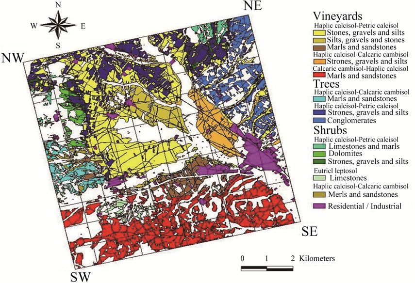
Figure 1. Map of soils over the 10 km × 10 km defined area.
is statistically different between units and homogeneous inside each one. This way, a representative soil moisture value of each area unit can be obtained sensing this parameter in just one point inside the unit. This methodology allows using a low number of sensors for covering the 10 km × 10 km area. Specifically, we will consider zones with vineyards, fruit trees and shrubs for locating the soil moisture sensors in order to get representative data. Consequently, position as well as number of sensors will be conditioned by both the soil type and use. As a trade off, we decided to install 12 sensing stations, with the following distribution: 5 sensors into vineyard lands (V1, V2, V3, V4 and V5), 3 sensors in fruit tree fields (T1, T2, T3) and 4 sensors over shrub zones (M1, M2, M3, M4). This way, all possible combinations of soil type/soil use are covered. Obviously, new nodes could be easily added to the network, if necessary.
2.2. Transmission Media
The selection of the transmission mechanism is hardly conditioned by the characteristics of the environment where a sensor network is developed [6]. In our case, the most of the region is open field, in a non urban environment. Consequently, the use of radio frequency based links becomes unavoidable. Among different available technologies and frequency bands (GSM, Bluetooth, WiFi, ···), we chose the 868 MHz ICM band. Even though GSM links should give the network a better ubiquity, the maintenance costs makes this option less attractive. Restricting to open radio bands, ICM-868 MHz is also a free band. Higher range links can be achieved with respect to 2.45 GHz bands, with low power requirements. In addition, once the network is implemented, the maintenance cost is extremely low, since data transmission is for free. As a first developing step, in order to ensure a radioelectrically free environment, electromagnetic field measurements were systematically performed in the Utiel-Requena plateau, mainly in the 868 MHz band. We concluded that the ICM band was free of saturation in the area, and so it could be used for our project.
2.3. Communications Hardware
The communication hardware consists, basically, of:
2.3.1. Radio Transmitter (Emitter/Receiver)
In order to modulate/demodulate the digital signal and then transmit it via radio, a transmitting/receiving commercial (Radiomodem Wlink8S from DMD [7]) was selected. This device operates in the ICM 868 MHz band with a FSK modulation. Besides, it offers high transmission power (up to 30 dBm) and good sensitivity (–97 dBm). These features are expandable by using external antennas, a power save mode with low current consumption (only 2.5 mA) and a typical power supply (3.6 V to 6 V). The transmitter is controlled and programmed by single sequences of ASCII AT (ATtention) commands, through a RS-232 interface using a PC or a microcontroller. Every device has a number or identification name. When two radiomodems are in the same area of influence, a direct communication is stated.
2.3.2. Antennas
For increasing the range of the links, we are forced to use external antennas. Two types of antennas are chosen according to their radiation pattern. Both will be used depending on the position of the particular node. We used omnidirectional antennas with a gain of 7.3 dBi (GP-901, by SIRIO) and directional Yagi antennas with a gain of 12.0 dBi (SY-910, by SIRIO) [7].
2.3.3. Link Calculations
Once the radio frequency module and the antennas were chosen, we estimated the respective link ranges, paired considered, assuming conditions of free space and direct vision between antennas, and without considering several attenuations like obstacles, meteorological inclemencies, interferences, diffractions, etc. [8]. By knowing the emitter power (10 dBm), the receiver sensitivity (–97 dBm) and the antennas gain, we can calculate the maximum distances between a possible emitter and a receiver using the radio link balance equations. For a link between two omnidirectional antennas, we have a maximum range close to 5 km. For a link between an omnidirectional antenna and a directional one, the maximum range is about 8 km.
2.4. Network Topology
The final network implementation needs to take into account the defined units, the zone relief and the maximum ranges previously between links. Taking advantage of a small mountainous elevation with direct vision of the most of the region, and after considering different possible topologies [9], we decided to establish this point as the central node of the network. From it, the other nodes would be linked as ramifications with a hierarchic form. This point belongs to the unit defined as M4. With the obtained link calculations, the radio frequency module and the antennas, distances of about 12 km would be achieved by using an intermediate node. After numerous field observations, specific link measurements, and always conditioned by the type and use of the soil, the most effective network structure is that shown in Figure 2.
Each link was individually calculated and measured. The summary of the main parameters of the link tests are shown in Table 1. Measured distance between nodes (as calculated from UPS positions) as well as estimated (ST) and measured (SE) sensitivities are also displayed. Notice that only nodes M4 and V1 need omnidirectional antennas (so, link M4-V1 is the more restrictive).
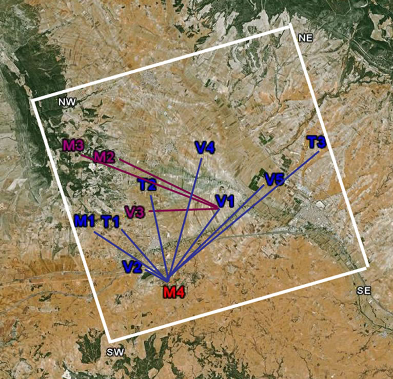
Figure 2. Node positions and links on the 10 km × 10 km area.


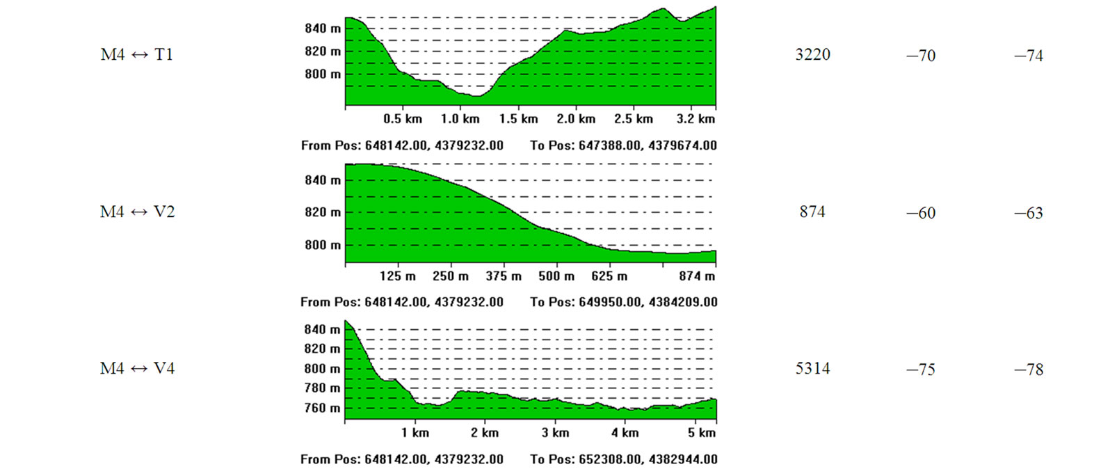
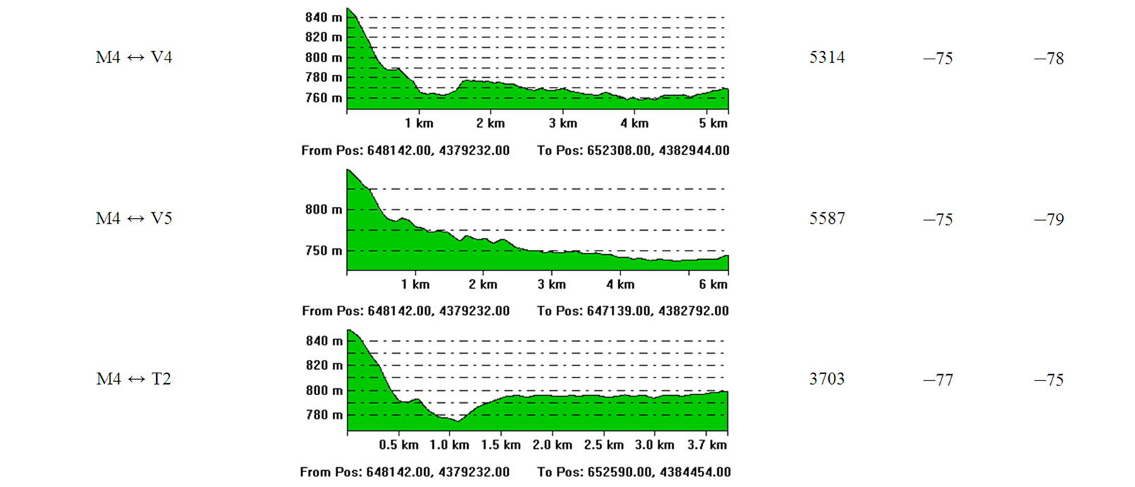
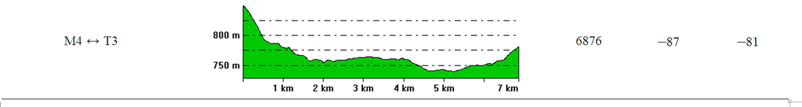
Table 1. Table type styles (Table caption is indispensable).
3. Sensor Node
After choosing the communication system, deciding network topology and fixing the position of the nodes, the hardware and software of each one and the development of the communication protocol is now explained. Each node is equipped with necessary electronics in order to provide soil moisture measurements, store the acquired data and control the communication with other sensors.
3.1. The Hardware
A simplified block diagram of a sensor node is shown in Figure 3. Apart from the communications hardware, a node basically consists of a battery-based power supply, a soil moisture sensor, an acquisition and control board and a memory system.
3.1.1. Power Supply
The nodes need to be independently fed by means of solar cell operated batteries, due to the difficulty of accessing the mains in every node of the network. Specifically, we have made use of a MSX 01F (BECOsolar) solar cell (1 W of nominal power) [7] and four series NiMh rechargeable batteries with a capacity of 1800 mAh and 4.8 V of nominal voltage. The charge ratio is up to 90 mAh under good solar radiation conditions. These batteries directly feed the RF module. Regarding the acquisition and control electronics board, as well as for the soil moisture meter, a DC-DC converter is necessary in order to supply the required +5 V. For this purpose, a voltage elevator, together with a voltage regulator was specifically designed and implemented.
3.1.2. Soil Moisture Sensor
The soil moisture was measured by means of a ThetaProbe ML2x (Delta-T Devices) [8]. This is a capacitive probe that estimates the amount of volumetric humidity from dielectric constant measurements. The output is a DC differential voltage, ranging from 0 V to 1 V for a relative dielectric constant value ranging from 1 to 32, corresponding to a 0.5 m3/m3 amount of volumetric

Figure 3. Simplified block diagram of a sensor node.
humidity of the soil. The conversion relationship depends on the soil characteristics and needs to be calibrated for any particular case. The probe can be fed with a voltage between +5 V and +15 V. Because the probe does not need to be continuously measured, it is connected/disconnected through a typical common emitter transistor.
3.1.3. Acquisition, Conditioning and Control System
For monitoring medium-scale sensor networks, a microcontroller based architecture has been proved to be powerful enough [9]. For this particular case, each node is controlled by a PIC16F876 (Microchip) microcontroller, with the following assigned tasks:
(1) Acquisition of the measured data, provided by the soil moisture sensor, through an A/D port. The differential voltage needs to be previously converted to a 0 V/+5 V level by means of a specific instrumentation amplifier together with an operational amplifier;
(2) Acquisition of the ambient temperature, through a digital integrated thermometer (DS1631) connected to the I2C bus;
(3) Monitoring of the battery charge voltage status through an additional A/D port;
(4) Communication with the RF module, making use of the Universal Asynchronous Receiver Transmitter (UART). For this purpose a RS-232/TTL level converser (MAX3222, Maxim) equipped with a shutdown (low consumption) mode was specifically designed and implemented;
(5) Synchronization of the network, with an external Real Time Clock (RTC), controlled through the I2C bus. We have selected the DS1678 (Maxim). The RTC also interrupts periodically the microcontroller, with a configurable alarm, to start a new measurement.
3.1.4. Memory System
For the data storage, a 512 kbit I2C controlled external EEPROM is utilized. If a particular data ratio of a measurement every ten minutes is considered, this memory allows a backup communication failure protection of 7 days in the worst case (if the failure is of the central node) or a maximum of 84 days (end node failure).
3.2. The Software
3.2.1. Communication Protocol
For a proper function of the network, all nodes must be synchronized in order to correctly correlate the measurements as well as to optimize the communication protocol by reducing unnecessary waiting times. In the network, each node will be identified by a unique software address. These nodes should operate in a standby (low power consumption) mode when neither measurement nor transmission activity is required. The whole network will be regulated by a PC, directly connected to the central node. This particular node will initialize the network, synchronize it, and store the data collected from all the nodes. Additionally, an error detection/correction protocol is also considered in this communication system.
In this sense, a Medium Access Control (MAC) based protocol [10], adapted to hierarchic networks has been developed. The transmitted ASCII messages are arranged in a particular format, containing the fields: origin and target address, type of command, data length, message identifier and error checking.
Commands fall in one of the following categories:
(1) Transmission acknowledgement (ACK/NACK);
(2) Shutdown activation/deactivation;
(3) Measurement start;
(4) Data asking;
(5) Data sending;
(6) Synchronization;
(7) Reset.
Initially, the network is in a standby state. A personal computer, directly connected to the central node, initializes the network. Then, synchronization and start measurement commands are sequentially sent to the network. These commands travel hierarchically through the network until reaching all the nodes. Sometime after, and in the same way, the computer sends commands asking for data. Then, the stored data from the performed measurements travel back from the end nodes to the central one. All the data are then organized by the PC, allowing the subsequent analysis.
3.2.2. Acquisition
At a certain time a given node receives a synchronization order and a start measurement command. In response, the microcontroller configures the RTC and states an alarm that will be activated each time a measurement must be made. This way the node is periodically capturing the defined measurements and storing them in the EEPROM, together with the clock information. At any time, a node can receive a command asking for data. In this case, the node will send the stored data to the upper level node. For clarity, In Figure 4, a summarized software flux diagram is shown.
3.3. Power Consumption
The protocol is energy optimized by properly using the shutdown mode. In this sense, the communication time is highly minimized, leading to considerable energy savings. The averaged power consumption can be estimated as in [11]. Let’s consider a particular case consisting of making a measurement every 10 minutes and sending the data every hour. The complete measuring/receiving/transmitting process, as well as the summarized calculations, are detailed in Figure 5. From averaged statistical radiation
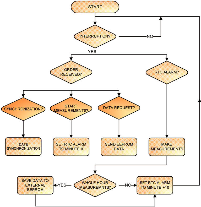
Figure 4. Software flux diagram.
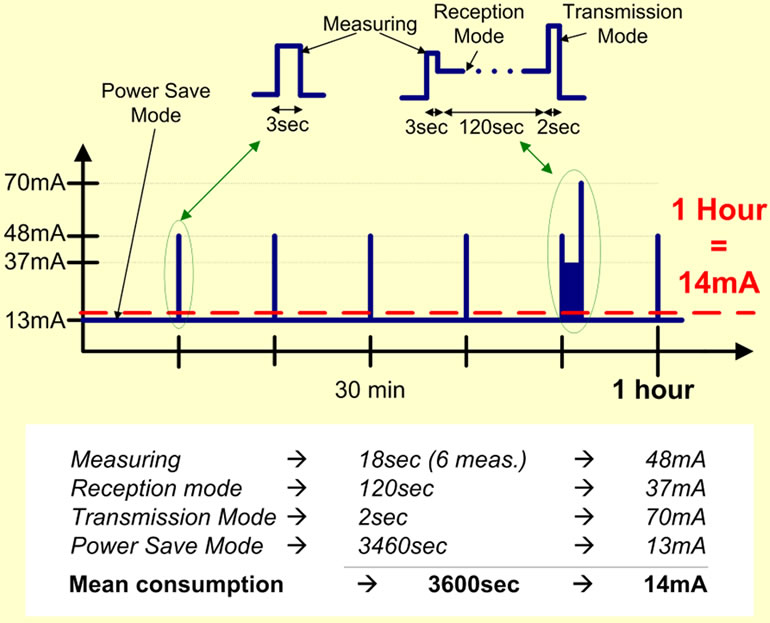
Figure 5. Power consumption scheme.
measurements over the considered region, and taking into account the characteristics of the utilized solar cell, the averaged charge of the battery of a node can be estimated to be about 480 mAh. From data in Figure 5, the consumed energy in a day should be 336 mAh (14 mA × 24 h). Therefore, the energetic balance should be always positive. Moreover, the functionality lifetime of every node, from an energetic point of view, would be of more than 5 (absolutely dark) days.
4. Implementation
The final node implementation is depicted in Figure 6. The RF module (highlighted in green) as well as the electronics board (highlighted in orange) and the batteries (below the RF module) are installed into a watertight box. The solar cell is placed onto the box enclosure. The letters correspond to those used in Figure 3.
The box is then attached to a 3-meter mast, also holding the antenna, and close to it. The particular arrangement and final installation configuration hardly depends on the ground conditions, as we try to show in Figure 7. In Figure 7(a), we can see an “omnidirectional type” node installed onto the wall of an existing small construction over vineyards. In Figures 7(b) and (c), the mast of a “directional type” node must be directly installed onto the ground over trees and shrubs respectively, with the help of tensors.
5. Results
The diagram of the overall system is shown in Figure 8. As explained before, all collected data are centralized by a PC, connected to Internet. This way, the soil moisture data access can be done by different devices through internet and the data server.
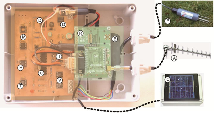
Figure 6. Detailed sensor implementation.

Figure 7. Sensing node implementation: (a) Over a vineyard field; (b) Over an olive tree field; (c) Over a shrub area.

Figure 8. Data access configuration.
As easily observed, the soil moisture (Figure 9) varies with several significant rain events. The different drying processes suggest dependence with the soil characteristics and land uses, assuming a homogeneous amount of rain inside the reference area. In Figure 10, the typical evolution of the temperature is displayed. The day-tonight variation is clearly highlighted. Additionally, an example of the battery charge monitoring is also shown in Figure 11. If we correlate this date with those in Figure 10, we can extract that the battery discharge is more appreciated in the rainy days, when the clouds difficult the solar cells function. During these rainy days, the clouds also produce a smoothing of the temperature variations. These considerations are included only as illustrative examples of the potentiality of the collected data.
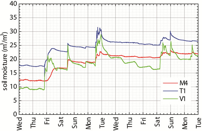
Figure 9. Measured volumetric soil moisture.
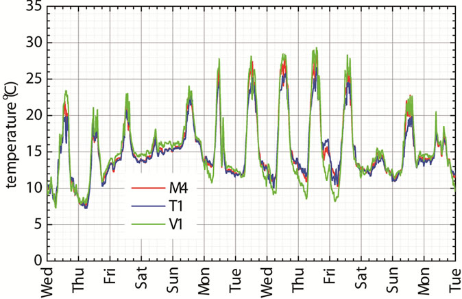
Figure 10. Measured ambient temperature.
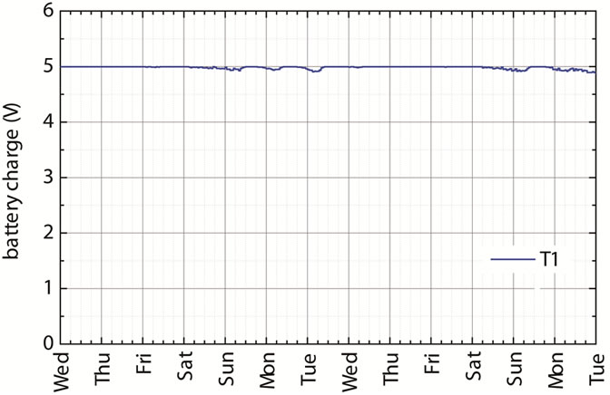
Figure 11. Measured battery charge.
6. Conclusions
We have successfully designed and implemented a completed sensor network for soil moisture monitorization using radio links in a wide 10 km × 10 km reference area. By sampling each defined unit, a low density of sensors has been achieved. This fact has allowed us to cover a higher area with lower cost of implementation.
The network, once configured, is automatic. It makes use of radiofrequency 868 MHz RF modules with a hierarchical configuration capable to cover the whole area with radio-links up to about 7 km.
Each node is equipped with a soil moisture probe and a microcontroller based electronics board in order to capture and store the environmental data, at the desired intervals. A solar cell supplies the power to a rechargeable battery, allowing the system to be autonomous.
A central node, directly connected to a PC, is dedicated to configure and control the network, as well as to collect the data from all the nodes and to allow their access through Internet from anywhere. This way, we have completed a typical sensor network including a real time web application to access the soil moisture data.
The system is fault tolerant, and immediately extensible to a higher number of nodes in a wider region, or to the measurement of additional environmental variables.
REFERENCES
- L. Min-Hui and S. J. Famiglietti, “Precipitation Response to Land Subsurface Hydrologic Processes in Atmospheric General Circulation Model Simulations,” Journal of Geophysical Research-Atmospheres, Vol. 116, 2011, Article ID: D05107.
- S. Mecklenburg, M. Drusch, Y. Kerr, J. Font, M. MartinNeira, S. Delwart, G. Buenadicha, N. Reul, E. DaganzoEusebio, R. Oliva and R. Crapolicchio, “ESA’s Soil Moisture and Ocean Salinity Mission: Mission Performance and Operations,” IEEE Transactions on Geoscience and Remote Sensing, Vol. 50, No. 5, 2012, pp. 1354-1366. doi:10.1109/TGRS.2012.2187666
- European Space Agency, “SMOS Earth Explorers,” 2012. http://www.esa.int/esaLP/LPsmos.html
- E. López-Baeza, A. Velázquez, C. Antolín, A. Bodas. J. F. Gimeno, K. Saleh, F. Ferrer, C. Domenech, N. Castell and M. A. Sánchez, “The Valencia Anchor Station, a cal/ val Reference Area for Large Scale Low Spatial Resolution Remote Sensing Data And Products,” Proceedings of Symposium on Recent Advances in Quantitative Remote Sensing, Valencia, 16-20 September 2002, pp. 16-20.
- C. Millán-Scheiding, C. Antolín, A. Cano and E. LópezBaeza, “The Use of Physio-Hidrologic Units for Soil Moisture Monitoring with SMOS,” III National Symposium on Desertification and Soil Degradation, September 2007.
- W. T. Davis, X. Liang, C.-M. Kuo and Y. Liang, “Analysis of Power Characteristics for Sap Flow, Soil Moisture, and Soil Water Potential,” IEEE Sensors Journal, Vol. 12, No. 6, 2012, pp. 1933-1945. doi:10.1109/JSEN.2011.2179933
- Digital Micro Devices (DMD), “Products,” 2012. http://www.dmd.es/
- Delta-T Devices, “Products,” 2012. http://www.delta-t.co.uk/
- M. Keshtgari and A. Deljoo, “A Wireless Sensor Network Solution for Precission Agriculture Based on Zigbee Technology,” Wireless Sensor Network, Vol. 4, No. 1, 2012, pp. 25-30. doi:10.4236/wsn.2012.41004
- F. Ianello, O. Simeone and U. Spagnolini, “Medium Access Control Protocols for Wireless Sensor Networks with Energy Harvesting,” IEEE Transactions on Communications, Vol. 60, No. 5, 2012, pp. 1381-1389. doi:10.1109/TCOMM.2012.030712.110089
- M. Pandey and S. Verma, “Energy Consumption Patterns for Different Mobility Conditions in WSN,” Wireless Sensor Network, Vol. 3, 2011, pp. 378-383. doi:10.4236/wsn.2011.312044
NOTES
*Corresponding author.