ABSTRACT

This paper reports on the current state of surface water and ocean contamination models—based on the needs of US Government agencies, their Information Technology (IT) systems, and business processes. In addition, down-selection and evaluation criteria were applied in a two-step process. In Step 1, sixty five surface water and ocean models were identified and researched. In Step 2, the following criteria were explored for each model: 1) model environment (river, lake estuary, coastal ocean and watershed); 2) degree of analysis (screening model intermediate model, advanced model); 3) availability (public domain, proprietary); 4) temporal variability (steady state or time variable/dynamic); 5) spatial resolution (one, two or three dimensional); 6) processes (flow, transport, both flow and transport in an integrated system); 7) water quality (chemical, biological, radionuclides, sediment); and 8) support (user support/training available, user manuals/documents available).

1. Introduction

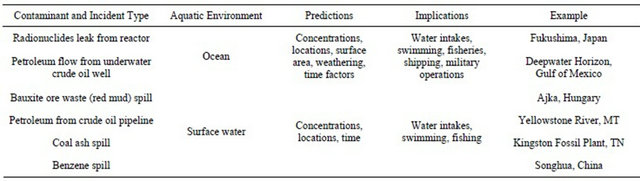
The purpose of this project was to research and report on the current state of surface water and ocean water contamination models. Environmental analysts require estimates of water contamination levels and expected dispersion/transport patterns following intentional or accidental chemical (including crude oil and petroleum products) and radiological releases to aquatic environments. Water contamination modeling assists in assessing potential impacts to human/environmental health and government operations by providing predictive estimates of contaminant concentration, speed and direction of travel. Examples of recent water contamination incidents which are of interest are listed in Table 1.

Water quality modeling has evolved significantly in the last century. The period from 1850 to 1930 was the period of scientific and quantitative understanding of the hydrologic cycle and its processes [1]:

• Mulvaney: 1851—Development of concept of time of concentration.

• Darcy: 1856—Established basic law of groundwater motion.

• St. Venant: 1871—Derived the equations of one-dimensional surface water flow.

• Manning: 1891—Developed an equation for open channel flow velocity.

• Green and Ampt: 1911—Development of infiltration model.

Streeter and Phelps: 1925—Developed the dissolved oxygen sag curve for rivers.

The frequency of these events (Table 1) is rare, their impacts are high, and their occurrence is hard to predict. The modeling of the above mentioned events have many associated unknowns. The following characteristics make the event challenging from the modeling perspective.

• Unknown site characteristics—location, soil characteristics, land use, etc.

• Unknown sources of contamination—point or polygon.

• Unknown release rate of contaminants—instantaneous or continuous.

• Unknown deposition rate of contaminants—dry deposit or wet deposit.

• Unknown parameters for data—availability and accessibility of data; sources of data; format of data.

Until the 1960s, the scope of the problems that could be solved was constrained by the computational tools available [2]. The advent of digital computers led to major advances in modeling. Water quality model development and complexity kept pace with the advances in computers. The first advancement in the 1960s was the extension of simple 1-dimensional models to 2-dimensional modeling. This was followed by biological modeling (eutrophication) and then multi-dimensional and multi-species modeling. The period since 1980 has seen

Table 1. Examples of water contamination modeling needs.

the development of user-friendly, GIS-linked hydrologic, hydraulic and water quality models, and extensive use of these models in a variety of applications.

This report focuses on riverine, estuarine, and coastal ocean water contamination modeling and addresses three major components that are important to government agency consideration for model selection, evaluation and implementation:

• Riverine, estuarine, and/or coastal ocean contaminant model.

• Input data for the model.

• Expertise required to run the model and interpret the results.

2. Information and Data Collection

Our first task was to identify and collect information on surface water and ocean contamination models. Water contamination models are developed by many Federal, State, and local agencies, as well as universities, private companies, and non-government organizations. These models were developed for many purposes and by various methods, with varying levels of detail, accuracy and quality. There are literally hundreds of water quality models available. While the number of models is staggering, the fundamental concepts on which they are based are similar. Water quality models represent the following:

• The hydrodynamic flow fields that drive the movement of the water quality constituents.

• The movement and transformations of the water quality constituents.

The large number of models arises from different combinations of these parameters and assumptions and (often minor) differences in the algorithms used to represent particular processes as follows:

• Model Environment—River, Lake, Estuary, Coastal Ocean and Watershed.

• Degree of Analysis—Models are developed at various levels of complexity, depending on the application needs. The simplest models provide general predictions based on a limited set of environmental or physical factors. The most sophisticated models will solve fundamental equations on a detailed spatial and temporal scale. These models may be integrated with a geographic information system (GIS) which is used to provide spatially-arrayed input data or to spatially display the model results.

o  Screening models use empirical model/analytical methods for contaminant transport.

o  Intermediate models—These are hybrid models that do not require a rigorous mathematical solution.

o  Advanced models—Models that approximate a solution of governing partial differential equations that describe a natural process. The approximation uses a numerical discretization of the space and time components of the system or process. The advanced models use the following solution techniques for solving the system of equations; Finite Difference; Finite Element; Finite Volume; Harmonic Models (best for tidal basins); Methods of Characteristics (Eulerian-Lagrangian Models); Random Walk and Random Flight Particle Tracking.

• Availability—Public Domain, Proprietary, Restricted Support (support only for the developing organization).

• Temporal Variability—Steady State or time variable/ dynamic.

o  Steady state model—Mathematical model of fate and transport that uses temporally constant values of input variables to predict constant values of receiving water quality concentrations.

o  Time variable model—A mathematical formulation describing the physical behavior of a system or a process and its temporal variability.

• Spatial Resolution—Models may be one-, twoor three-dimensional. One-dimensional models are the most common type and generally the easiest to use but may not provide sufficient spatial representation in some cases.

o  One-dimensional models are limited to the simulations of cross-sectional averages generally based on the use of the Chezy or Manning equation to specify friction losses and the use of the dispersion coefficient of mixing to quantify mixing. They cannot effectively model steep slopes and stratified exchange of fresh and sea water.

o  Two-dimensional models explicitly represent variations in two dimensions. This may be x-y representation with complete mixing in the z-direction, x-z representation with complete mixing in the y-direction (estuaries), or y-z mixing with complete mixing in the x direction. 2-D horizontal plane models simulate estuaries as well mixed vertically. They represent lateral and longitudinal variations in velocity and constituent concentration for estuaries with non-uniform widths. 2-D models explicitly represent variations in two dimensions with the third dimension assumed to be completely mixed.

o  Three-dimensional models explicitly represent movement, variations and transformations in x-y-z space.

• Processes—Flow, Contaminant Transport, both Flow and Transport in as an integrated system.

o  Flow model—Calculates hydrology and hydrodynamic conditions (flow, velocity, surface runoff) which are then used as input to a water quality transport model.

o  Transport model—calculates the movement and transformation of water quality constituents.

o  Both—Hydrologic/hydrodynamic and transport models are integrated into a single Model.

• Water Quality—Chemical, Biological, Radionuclides, Sediments.

• Support—User Support/training available, User Manuals/documents available.

3. Model Review Methodology

The model review consisted of a two-step process (model identification and summarization of capabilities):

Step 1. Model Identification—The search for available models for river and ocean contamination was initiated by literature review. A comprehensive list of models was developed. The review included the following sources:

• USEPA Water Quality model use database.

• USEPA Council for Regulatory Environmental modeling.

• USACE Environmental Laboratory.

• USGS—The Surface Water and Water Quality Models Information Clearinghouse (SMIC).

• Water Environment Research Foundation (WERF).

• UNESCO.

• Ministry of Environment, Parks, and Land (British Columbia, Canada).

• National Council on Radiation Protection and Measurements.

• Open Literature.

• http://www.ncasi.org/programs/areas/water/emrg/werf_aera.htm.

• http://smig.usgs.gov/SMIG/model_archives.html.

Step 2. Summarization—The models were summarized based on the information available from the literature and the criteria presented in Table 2 below.

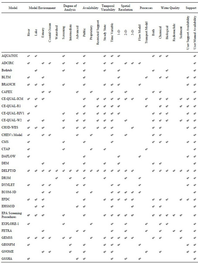
The results are shown in Tables 3 and 4. Table 3 provides the acronyms, names, and availability information of the water contamination models that were identified in the literature review. The salient features and functionality of the available models is summarized in Table 4.

4. Development of Model Selection Criteria

The proper selection of a model is essential to the successful simulation of water contamination modeling. Model selection is the first step in a modeling task. As shown in Tables 3 and 4, there are numerous riverine and ocean water models available. Government requirements can be met with a suite of models appropriate for riverine, estuarine, and the coastal ocean environment.

Table 2. Model selection criteria.

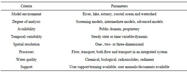
Table 3. Summary table of model names, references and availability.

Continued

Continued

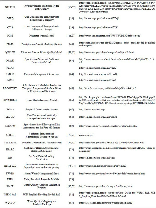
Table 4. Comparative features and functionality of water contamination models.

Continued

The selection of these models is based on meeting a specific modeling objective (e.g., a toxic spill in a river affecting drinking water supplies downstream).

The major differentiators between the models identified in this report is the way they handle spatial and temporal dimensions and how they model the fate and transport processes. Not all models, however, are appropriate under all conditions. They vary greatly with respect to their analytical approach, underlying assumptions, data needs, and output capacity. The process of selecting a model is not limited to evaluating the model science. The level of sophistication required in a modeling study reflects constraints such as:

• Accuracy required.

• Allotted time frames for study completion.

• Availability and reliability of input data.

• Training and expertise required for model operation.

These constraints and others combine to determine whether modeling is an appropriate tool for achieving the objectives, which model is the best choice for application and the limitations in interpreting the model results. Confidence in model results is based on the quality of data used to construct the model, the capabilities of the modeler, and the proven ability of the model to simulate observed phenomena [84]. For the development of the model selection criteria, issues addressed by the National Research Council [85], Environmental Protection Agency [86] and criteria discussed in the literature were reviewed. The following three issues were addressed in developing the model selection criteria:

• Model characteristics.

• Input data.

• Technical expertise.

4.1. Model Characteristics

The choice of the appropriate level of model complexity is determined in large measure by the nature of problem. The ability to model the transport, transformation and fate of sediments and interacting contaminants in surface water systems rests upon the ability to select a model or models which appropriately represents the most significant processes controlling the system. Since model studies are most often conducted under economically imposed constraints, including personnel, model software availability, computer hardware limitations, and the availability of field data for model calibration and validation, modeling strategies often necessitate selection of a model which meets minimum, but acceptable, criteria for process representation. The model selection criteria are organized into three categories as described below:

Application criteria specify the nature and intent of the analysis to be performed. The application criteria for model selection are based primarily on:

• Consistency of the model with the scientific theory.

• Model appropriateness for the complexity of the problem.

• Identification of the problem.

• Relationship of the model to the problem.

• Availability in public domain.

Technical criteria specify the site-specific processes to be simulated by the model. The technical criteria for model selection are based primarily on:

• Physical mixing and transport processes.

• Biological, chemical, and physical degradation and transformation processes.

• Geometry and/or dimensionality and time variability of the system.

• Temporal and spatial scales and extent of the models.

• Content, accuracy, currency and resolution of data available for modeling.

• Quantification of the uncertainty.

• Model is consistent with the amount of data available.

• Solution scheme examination.

• Model calibration and validation.

• Compatibility with Geographic Information System (GIS).

• Ease of output comprehension (e.g. graphs, maps, etc.).

Operational criteria specify the quality assurance (QA) and documentation requirements. The operational criteria are related to the degree of quality assurance (QA) and documentation to which a model has been subjected.

• Availability of test problems for comparison either in the user’s manual or from the source where the model was obtained.

• Proven track record for the model—model must have been applied and calibrated to real world problems rather than have been developed and applied in theoretical hypothesis testing.

• Flexible for future updates and improvements.

• Cost for annual model support is an acceptable longterm expense.

4.2. Input Data to Support the Model

The model data plays a crucial role in the model selection process. For water contamination modeling, three types of data are required.

• Input data.

• Data for calibrating the model.

• Data for validating the results.

Issues pertaining to assembling and entering data into the model include the following:

• Existence of data.

• Collection of data (data collection is a resource intensive exercise which can be a critical factor during emergencies).

• Availability of data (public vs. proprietary; classified vs. unclassified).

• Accessibility of data (hardcopy vs. electronic).

• Format of the data (pre-processing of data in model compatible format).

4.3. Expertise of the Modeler

A typical modeling application requires data collection, data preparation, model simulations, results interpretation, and model reporting. All these steps are dependent on the expertise of the modeler. Expertise of the modeler will have a major impact on model results.

Staff resources are also a major consideration in modeling. Familiarity of the modeler with a particular type of model (e.g., finite element versus finite difference), or direct experience with a model sometimes get considered as a factor in the model selection. But in no case, however, should familiarity with a model dictate its selection when it does not satisfy the objective, technical, and implementation criteria.

5. Summary and Conclusions

5.1. Model Evaluation Criteria

Modeling strategies often necessitate selection of a model which meets minimum but acceptable evaluation criteria. The current model evaluation criteria are based on the information collected and analyzed. The evaluation criteria include the following:

Application Evaluation for model selection consists of the following parameters:

• Model/software availability and cost.

• Computer hardware limitations.

• Methods—Modeling approaches for the major processes flow, chemical fate and transport processes.

• Output—Type of outputs and output options, Level of outputs.

• User Interface—Input helpers, windows based or raw edits of input files, GIS interface for data.

Technical Evaluation for the model selection includes the following parameters:

• Model Environment—River, lake, estuary, ocean, watershed.

• Degree of Analysis—Screening, intermediate, advanced.

• Availability—Public, proprietary.

• Type—Steady state, dynamic.

• Level of Complexity—1-D, 2-D, 3-D.

• Processes—Flow, transport, both.

• Water Quality—Chemical, biological, radiological, sediment.

• Scale—Spatial, temporal.

• Input data required for model simulation, calibration and validation.

• Data—Data requirements and sources, level of accuracy of the data.

Operational Evaluation for the model selection includes the following parameters:

• Supporting Materials—Example input and output data sets, Identification of sensitive input parameters, calibration procedures for field measurements, continuing education and training.

• Availability and user friendliness of the interface for ease of input preparation.

• GIS linkage—for large modeled areas.

• Model Availability—Model contacts, documentation, source availability, version tracking.

5.2. Data as Evaluation Criteria

For Outside the Continental United States (OCONUS) riverine, estuarine, and ocean modeling applications, data can be a limiting factor.

• Availability of data in foreign countries can be a limiting factor, especially in regions of conflict. For example, no hydrological data has been collected in Afghanistan after 1979.

• Collection and preparation of data even for a simple model requires time. This is particularly important in emergency situations where fate and transport of contaminants is required immediately for a proper response. Therefore, focus on data should also be an important factor in model selection.

• Language is a major barrier for data collection in foreign countries. Usually countries collect data in their national language and rarely is it available online or translated into the English language.

• Data may be collected only for the main reaches of major rivers or estuaries. Data for other hydrological parameters (depth, width, velocity, roughness coefficients etc.) may not available.

• In many developing countries data is not freely available. In many countries because of unresolved transboundary issues data is not freely distributed.

• In developing countries hydrologic data is more available than water quality data because of resource development and management.

5.3. Technical Expertise as Evaluation Criteria

Technical expertise of the modeler should be considered as part of the evaluation criteria. The modeler is the human interface in the whole modeling exercise. The modeler not only runs the model but also calibrates the model, validates the results, and interprets the output. The following criteria should be considered for the technical expertise evaluation:

• Level of technical expertise needed to run the selected model.

• Manpower required to run the model.

• Training requirements.

• IT support for the model.

5.4. Additional Criteria

A critical requirement of several government agencies is to acquire the capability to model “unusual events” in the aquatic environment. These “unusual events” have certain modeling and data unknowns as illustrated below. These unknowns are the limiting factors for model selection.

• Site characteristics.

• Sources of contamination—point, polygon, instantaneous, continuous.

• Release rate of contaminants.

• Deposition rate of contaminants.

• Data.

o  Availability and accessibility of data.

o  Sources of data.

o  Format of data.

6. Acknowledgements

The authors wish to thank Dr. Alan Blumberg and Dr. Walter Grayman for their comments, reviews and suggestions regarding this study.

REFERENCES

- D. R. Maidment, “Handbook of Hydrology,” McGraw-Hill, Inc., New York, 1992, p. 1992.
- S. C. Chapra, “Surface Water Quality Modeling,” McGrawHill Inc., New York, 1997, p. 844.
- EPA, “AQUATOX for Windows: A Modular Fate and Effects Model for Aquatic Ecosystems (Release 1), Vol. 3,” Model Validation Reports, Office of Water, Washington DC, 2000.
- R. A. Luettich Jr., J. J. Westerink and N. W. Scheffner, “ADCIRC: An Advanced Three-Dimensional Circulation Model for Shelves Coasts and Estuaries, Report 1: Theory and Methodology of ADCIRC-2DDI and ADCIRC-3DL,” Dredging Research Program Technical Report DRP-92-6, US Army Engineers Waterways Experiment Station, Vicksburg, 1992, p. 137.
- W. W. Walker, “Empirical Methods for Predicting Eutrophication in Impoundments: Report 3, Phase III: Model Refinements. Technical Report E-81-9,” US Army Engineer Waterways Experiment Station, Vicksburg, 1985.
- W. W. Walker, “Empirical Methods for Predicting Eutrophication in Impoundments; Report 3, Phase III: Applications Manual. Technical Report E-81-9,” US Army Engineer Waterways Experiment Station, Vicksburg, 1986.
- H. E. Jobson, “Enhancements to the Branched Lagrangian Transport Modeling System,” US Geological Survey, Reston, 1997.
- H. E. Jobson and D. H. Schoellhamer, “Users Manual for a Branched Lagrangian Transport Model,” US Geological Survey, Reston, 1987.
- R. W. Schaffranek, “Flow Model for Open-Channel Reach or Network,” U.S. Geological Survey Professional Paper 1384,” 1987, p. 12.
- J. D. Wang and J. J. Connor, “Mathematical Modeling of Near Coastal Circulation, Report No. 217,” Massachusetts Institute of Technology, Department of Civil Engineering, Cambridge, 1975.
- C. F. Cerco and T. Cole, “User’s Guide to the CE-QUALICM Three-Dimensional Eutrophication Model, Release Version 1.0, Technical Report EL-95-15,” US Army Engineer Waterways Experiment Station, Vicksburg, 1995:
- Environmental Laboratory, “CE-QUAL-R1: A Numerical One-Dimensional Model of Reservoir Water Quality; Users Manual, Instruction Report E-82-1,” US Army Engineer Waterways Experiment Station, Vicksburg, 1986.
- Environmental Laboratory, “CE-QUAL-RIV1 (ver 2): A Dynamic One-Dimensional (Longitudinal) Water Quality Model for Streams, User’s Manual, Instruction Report,” US Army Corps of Engineers Waterways Experiment Station, Vicksburg, 1995.
- T. M. Cole and E. M. Buchak, “CE-QUAL-W2: A TwoDimensional, Laterally Averaged, Hydrodynamic and Water Quality Model, Version 2.0. Technical Report EL- 95-1,” US Army Corps of Engineers, Waterways Experiment Station, Vicksburg, 1995, p. 75.
- Environmental and Hydraulics Laboratories, “CE-QUALW2: A Numerical Two-Dimensional, Laterally Averaged Model of Hydrodynamics and Water Quality, Instruction Report E-86-5,” US Army Corps of Engineers Waterways Experiment Station, Vicksburg, 1986.
- Y. P. Sheng and H. L. Butler, “A Three-Dimensional Mathematical Model of Coastal, Estuarine and Lake Currents, Technical Memorandum, 82-07,” Aeronautical Research Associates, Princeton, 1982.
- H. S. Chen, “A Mathematical Model for Water Quality Analysis,” Proceedings American Society of Civil Engineers, Hydraulics Division, Specialty Conference on Verification of Mathematical Models and Physical Models in Hydraulic Engineering, American Society of Civil Engineers, New York, 1978.
- S. Fant and M. S. Dortch, “Documentation of a OneDimensional, Time Varying Contaminant Transport and Fate Model for Streams,” ERDC/EL TR-07-1, US Army Engineer Research and Development Center, Vicksburg, 2007.
- R. L. Doneker and G. H. Jirka, “CORMIX User Manual: A Hydrodynamic Mixing Zone Model and Decision Support System for Pollutant Discharges into Surface Waters,” EPA-823-K-07-001, 2007. http://www.mixzon.com/downloads/
- EPA, “Technical Guidance annual for Performing Waste Load Allocations, Book II Streams and Rivers, Chapter 3, Toxic Substances, EPA-440/4-84-022,” Office of Water Regulations and Standards, Washington DC, 1984.
- H. E. Jobson, “Users Manual for an Open-Channel Stream Flow Model Based on the Diffusion Analogy: US Geological Survey Water-Resources Investigations Report 89-4133,” US Geological Survey, Reston, 1989, p. 73.
- K. D. Feinger and H. S. Harris, “Documentation ReportFWQA Dynamic Estuary Model,” US Environmental Protection Agency, Water Quality Office, Washington, DC, NTIS No. PB 197 103, 1970.
- Deltares, 2012. http://www.deltaressystems.com/hydro/product/621497/delft3d-suite
- W. M. Alley and P. E. Smith, “Distributed Routing Rainfall-Runoff Model, Version II, US Geological Survey Open-File Report 82-344,” 1982, p. 233.
- USACE, “DYNLET Mode,” 2012. http://chl.erdc.usace.army.mil/chl.aspx?p=s&a=SOFTWARE;30
- A. F. Blumberg and G. L. Mellor, “A Description of a Three-Dimensional Coastal Ocean Circulation Model, in Three-Dimensional Coastal Ocean Models, Coastal and Estuarine Sciences,” AGU, Washington DC, 1987, pp. 1- 16.
- G. Mellor, “User’s Guide for a Three-Dimensional, Primitive Equation, Numerical Ocean Model,” Princeton University, Princeton, 1990.
- J. M. Hamrick, “A User’s Manual for the Environmental Fluid Dynamics Computer Code (EFDC),” Special Report 331, The College of William & Mary, Williamsburg, 1996.
- Y. P. Sheng, “A Three-Dimensional Mathematical Model of Coastal, Estuarine and Lake Currents Using Boundary Fitted Grid, Report. 585,” Aeronautical Research Association, Princeton, 1986.
- USEPA, “Water Quality Assessment: A Screening Procedure for Toxic and Conventional Pollutants,” Office of Research and Development, Athens, 1985.
- W. B. Mills, J. D. Dean, D. B. Porcella, S. A. Gherini, R. J. M. Hudson, W. E. Frick, G. L. Rupp and G. L. Bowie, “Water Quality Assessment: A Screening Procedure for Toxic and Conventional Pollutants. EPA-600/6-82-004a and b. Volumes I and II,” US Environmental Protection Agency, Washington DC, 1982.
- R. G. Baca, W. W. Waddel, C. R. Cole, A. Brandsetter, and D. B. Cearlock, “EXPLORE-1: A River Basin Water Quality Model,” Battelle Pacific Northwest Laboratories, Richland, 1973.
- Y. Onishi, “Sediment Contaminant Transport Model,” Journal of the Hydraulics Division, Proceedings of the American Society of Civil, Vol. 107, No. HY9, 1981.
- Y. Onishi, “Mathematical Simulation of Sediment and Radionuclide Transport in the Columbia River. BNWL- 2228,” Battelle Pacific Northwest Laboratories, Richland, 1977, p. 93.
- J. E. Edinger and E. M. Buchak, “Numerical Waterbody Dynamics and Small Computers,” Proceedings of ASCE 1985 Hydraulic Division Specialty Conference on Hydraulics and Hydrology in the Small Computer Age, American Society of Civil Engineers, Lake Buena Vista, 13-16 August 1985.
- K. O. Asante, G. A. Artan, S. Pervez, C. Bandaragoda, and J. P. Verdin, “Technical Manual for the Geospatial Stream Flow Model (GeoSFM): US Geological Survey Open-File Report 2007-1441,” US Geological Survey, Reston, 2008, p. 65.
- E. M. Buchak and J. E. Edinger, “Generalized, Longitudinal-Vertical Hydrodynamics and Transport: Development, Programming and Applications. Contract No. DA CW39-84-M-1636,” US Army Corps of Engineers Waterways Experiment Station, Vicksburg, 1984.
- C. J. Beegle-Krause, “General NOAA Oil Modeling Environment (GNOME): A New Spill Trajectory Model,” IOSC 2001 Proceedings, Tampa, 26-29 March 2001, pp. 865-871.
- C. W. Downer and F. L. Ogden, “Gridded Surface Subsurface Hydrologic Analysis (GSSHA) User’s Manual Version 1.43 for Watershed Modeling System 6.1,” 2006.
- Hydrologic Engineering Center, “HEC-HMS Hydrologic Modeling System User’s Manual, Version 3.5, Computer Program Document CPD-74A,” US Army Corps of Engineers, Davis, 2010.
- HEC, “HEC-RAS River Analysis System User’s Manual Version 4,” US Army Corps of Engineers Hydrologic Engineering Center, Davis, 2008.
- W. R. Waldrop and F. B. Tatom, “Analysis of the Thermal Effluent from the Gallatin Steam Plant during Low Flows, Report. 33-30,” Tennessee Valley Authority, Norris, 1976.
- E. J. Hayter and A. J. Mehta, “Modeling Cohesive Sediment Transport in Estuarial Waters,” Applied Mathematical Modelling, Vol. 10, 1986, pp. 294-303.
- E. J. Hayter, M. A. Bergs, R. Gu, S. C. McCutcheon, S. J. Smith and H. J. Whiteley, “HSCTM-2D, a Finite Element Model for depth-Averaged Hydrodynamics, Sediment and Contaminant Transport,” National Exposure Research Laboratory, Office of Research and Development, UE Environmental Protection Agency, Athens.
- B. R. Bicknell, J. C. Imhoff, J. L. Kittle Jr., A. S. Donigian Jr. and R. C. Johanson, “Hydrological Simulation Program-Fortran, User’s Manual for Version 11,” US Environmental Protection Agency, National Exposure Research Laboratory, Athens, 1997, p. 755.
- W. B. Samuels, R. Bahadur, M. Monteith, D. Amstutz, J. Pickus, K. Parker and D. Ryan, “NHD, RiverSpill and the Development of the Incident Command Tool for Drinking Water Protection (ICWater),” Water Resources Impact, Vol. 8, No. 2, 2006, pp. 15-18.
- J. P. Paul and J. A. Nocito, “Numerical Model for ThreeDimensional Variable Density Hydrodynamic Flows, Documentation of the Computer Program,” US Environmental Protection Agency, Duluth, 1985.
- J. P. Paul and J. A. Nocito, “Numerical Model for ThreeDimensional Variable Density Hydrodynamic Flows, Documentation of the Computer Program,” US Environmental Protection Agency, Duluth, 1989.
- K. W. Hess, “MECCA Programs Documentation,” NOAA Technical Report NESDIS 46, National Oceanic and Atmospheric Administration, Washington DC, 1989.
- Danish Hydraulic Institute, “MIKE 11 Reference Manual, Appendix A. Scientific Background,” Danish Hydraulic Institute, Hørsholm, 2001.
- Danish Hydraulic Institute, “MIKE 3 FM, User Guide and Reference Manual,” Danish Hydraulic Institute, Hørsholm, 2003.
- Danish Hydraulic Institute, “MIKE 21 Flow Model, Hydrodynamic Module, User Guide,” Danish Hydraulic Institute, Hørsholm, 2007.
- Danish Hydraulic Institute, “MIKE-SHE Volume I User Guide, User Guide,” Danish Hydraulic Institute, Hørsholm, 2007.
- D. R. F. Harleman, J. E. Dailey, M. L. Thatcher, T. O. Najarian, D. N. Brocard and R. A. Ferrara, “User’s Manual for the MIT. Transient Water Quality Network Model Including Nitrogen Cycle Dynamics for Rivers and Estuaries,” EPA-600/3-77-010, US Environmental Protection Agency, Corvallis, 1977.
- N. D. Katopodes and T. Strelkoff, “Two-Dimensional Shallow Wave Models,” Journal of Engineering Mechanics (ASCE), Vol. 105(EM2), 1979, pp. 317-114.
- N. D. Katopodes, “A Dissipative Galerkin Scheme for Open Channel Flow,” Journal of Engineering Mechanics (ASCE), Vol. 110(HY4), 1984, pp. 450-466.
- N. D. Katopodes, “Two-Dimensional Surges and Shocks in Open Channels,” Journal of Engineering Mechanics (ASCE), Vol. 110, No. 6, 1984, pp. 794-812. doi:10.1061/(ASCE)0733-9429(1984)110:6(794)
- R. L. Runkel, “One-Dimensional Transport with Equilibrium Chemistry (OTEQ): A Reactive Transport Model for Streams and Rivers,” US Geological Survey, Reston, 2010, p. 101.
- R. L. Runkel, “One-Dimensional Transport with Inflow and Storage (OTIS): A Solute Transport Model for Streams and Rivers,” US Geological Survey Water-Resources Investigations Report 98-4018, Reston,1998, p. 73.
- [61] G. H. Leavesley, R. W. Lichty, B. M. Troutman and L. G. Saindon, “Precipitation-Runoff Modeling System: User’s Manual,” US Geological Survey Water-Resources Investigations Report 83-4238, Reston,1983, p. 207.
- [62] S. C. Chapra, G. J. Pelletier and H. Tao, “QUAL2K: A Modeling Framework for Simulating River and Stream Water Quality, Version 2.07: Documentation and Users Manual,” Tufts University, Medford, 2007.
- [63] P. Shanahan, M. Henze, L. Koncsos, W. Rauch, P. Reichert, L. Somlyódy and P. Vanrolleghem, “River Water Quality Modeling: II. Problems of the Art,” IAWQ Biennial International Conference, Vancouver, 21-26 June 1998.
- [64] D. Mackay, S. Paterson and M. Joy, “A Quantitative Water, Air, Sediment Interaction (QWASI) Fugacity Model for Describing the Fate of Chemicals in Rivers,” Chemosphere, Vol. 12, No. 9-10, 1983, pp. 1193-1208. doi:10.1016/0045-6535(83)90125-X
- [65] I. P. King, “A Finite Element Model for Three Dimensional Flow, RMA 9150,” US Army Corps of Engineers Waterways Experiment Station, Vicksburg, 1982.
- [66] J. M. Boyer, S. C. Chapra, C. E. Ruiz and M. S. Dortch, “RECOVERY, a Mathematical Model to Predict the Temporal Response of Surface Water to Contaminated Sediment. Technical Report. W-94-4,” US Army Engineer Waterways Experiment Station, Vicksburg, 1994, p. 61.
- [67] E. Z. Hosseinipour and J. L. Martin, “RIVMOD, a OneDimensional Hydrodynamic and Sediment Transport Model, Model Theory and User’s Manual,” AScI Corporation at USEPA, Athens, 1992, p. 55.
- [68] A. F. Shchepetkin and J. C. McWilliams, “The Regional Oceanic Modeling System (ROMS): A Split-Explicit, FreeSurface, Topography-Following-Coordinate Oceanic Model,” Ocean Modeling, Vol. 9, No. 4, 2005, pp. 347-404. doi:10.1016/j.ocemod.2004.08.002
- [69] J. V. Letter Jr., L. C. Roig, B. P. Donnel, W. A. Thomas, W. H. McAnally and S. A. Adamec Jr., “Users Manual for SED2D-WES Version 4.3 Beta, a Generalized Computer Program for Two-Dimensional, Vertically Averaged Sediment Transport,” US Army Corps of Engineers Waterways Experiment Station Coastal Hydraulics Laboratory, Vicksburg, 1998.
- [70] C. D. Knightes, “Development and Test Application of a Screening-Level Mercury Fate Model and Tool for Evaluating Wildlife Exposure Risk for Surface Waters with Mercury-Contaminated Sediments (SERAFM),” Environmental Modeling& Software, Vol. 23, No. 4, 2007, pp. 495-510. doi:10.1016/j.envsoft.2007.07.002
- [71] C. K. Ziegler and B. S. Nisbet, “Long-Term Simulation of Fine-Grained Sediment Transport in Large Reservoirs,” Journal of Engineering Mechanics (ASCE), Vol. 121, No. 1, 1995, pp. 773-781. doi:10.1061/(ASCE)0733-9429(1995)121:11(773)
- [72] C. K. Ziegler and B. S. Nisbet, “Fine Grained Sediment Transport in Pawtuxet River, Rhode Island,” Journal of Engineering Mechanics (ASCE), Vol. 120, No. 5, 1994, pp. 561-576. doi:10.1061/(ASCE)0733-9429(1994)120:5(561)
- [73] Y. Onishi and S. E. Wise, “Mathematical Model SERATRA, for Sediment-Contaminant Transport in Rivers and Its Application to Pesticide Transport in Four Mile and Wolf Creeks in Iowa. EPA/600/3-82/045,” US Environmental Protection Agency, Athens, 1982.
- [74] Applied Science Associates, “System for Hazard Assessment of Released Chemicals, Version 1.0.0 User Guide,” Applied Science Associates, South Kingston, 2009.
- [75] SMS, 2012. http://www.scisoftware.com/environmental_software/detailed_description.php?products_id=119
- [76] J. J. Leenderste, “Aspects of a Computational Model for Long-Period Water-Wave Propagation, Memorandum Report No. RM-5294-PR,” US Air Force Project RAND, Rand Corp, Santa Monica, 1967.
- [77] J. J. Leenderste, “A Water Quality Simulation Model for Well Mixed Estuaries and Coastal Seas: Vol. 1, Principles of Computation, Report No. RM-6230-RC,” Rand Corp., Santa Monica, 1970.
- [78] J. J. Leenderste, “Aspects of SIMSYS2D, a System for Two-Dimensional Flow Computation, Report No. R- 3572-USGS,” Rand Corp., Santa Monica, 1987.
- [79] L. A. Rossman, “Storm Water Management Model User’s Manual Version 5.0. EPA/600/R-05/040,” US Environmental Protection Agency, Cincinnati, 2010. http://www.epa.gov/nrmrl/wswrd/wq/models/swmm/epaswmm5_user_manual.pdf
- [80] R. T. Cheng, V. Casulli and J. W. Gartner, “Tidal, Residual, Intertidal Mudflat (TRIM) Model and Its Applications to San Francisco Bay, California,” Estuarine, Coastal and Shelf Science, Vol. 36, No. 3, 1993, pp. 235-280. doi:10.1006/ecss.1993.1016
- [81] R. B. Ambrose Jr., T. A. Wool and J. L. Martin, “The Water Quality Analysis Simulation Program, WASP5, Part A: Model Documentation,” US Environmental Protection Agency Center for Exposure Assessment Modeling, Athens, 1993.
- [82] R. B. Ambrose Jr., T. A. Wool and J. L. Martin, “The Water Quality Analysis Simulation Program, WASP5, Part B: Model Documentation,” US Environmental Protection Agency Center for Exposure Assessment Modeling, Athens, 1993.
- [83] R. A. Schmalz, “User Guide for WIFM-SAL: A TwoDimensional Vertically Integrated, Time Varying Estuarine Transport Model,” US Army Corps of Engineers Waterways Experiment Station, Vicksburg, 1985.
- [84] Applied Science Associates, “WQMap User Manual, Version 5.0,” Applied Science Associates, South Kingston, 2004,
- [85] WERF, “Water Quality Models: A Survey and Assessment,” WERF Project#99-WSM-5, South Kingston, 2001.
- [86] NAP, “Assessing the TMDL Approach to Water Quality Management, Page 69,” National Academy Press, Washington DC, 2001. http://www.nap.edu/catalog/10146.html
- [87] US EPA, “Selection Criteria for Mathematical Models Used in Exposure Assessments: Surface Water Models,” US Environmental Protection Agency, Washington DC, 1987. http://nepis.epa.gov/Exe/ZyPURL.cgi?Dockey=30001GJB.txt