Journal of Water Resource and Protection
Vol.3 No.9(2011), Article ID:7522,11 pages DOI:10.4236/jwarp.2011.39077
Modelling of Streamflow of a Catchment in Kenya
Department of Environmental and Biosystems Engineering, University of Nairobi, Nairobi, Kenya
E-mail: jobiero@uonbi.ac.ke
Received July 1, 2011; revised August 4, 2011; accepted September 6, 2011
Keywords: Stream flow simulation, model evaluation, prediction, calibration and validation
ABSTRACT
Modeling stream flow forms a basis upon which policy makers, watershed planners and managers make appropriate decisions consistent with sustainable management of land and water resources in the watershed. The aim of this research is to provide a preliminary assessment of the performance of a complex watershed model in predicting stream flow on the Naro Moru river catchment in Ewaso Ng’iro river basin, Kenya. The research involved model input data preparation, model set up and test running, sensitivity analysis and calibration of the Soil Water Assessment Tool (SWAT) model. Preliminary evaluation of the model performance involved the use of known quantitative evaluation statistics that included correlation coefficient, Nash Sutcliffe efficiency (NSE), Deviation Volume (Dv) and a graphical technique for comparing observed and simulated flows. Initial model runs yielded poor daily flow simulations compared to monthly simulations. Poor daily simulation was attributed to differences in the timing of observed and simulated hydrographs. The model was calibrated for a three year period followed by a three year validation period based on monthly flows. Calibration results indicated an acceptable, but modest, agreement between observed and simulated monthly stream flows with a correlation coefficient (r) of about 0.7, NSE = 5%, and Dv = 61.7%. After validation, the model performance was satisfactory with the coefficient of determination (R2 ≈ 0.6), Nash-Sutcliffe efficiency (NSE) of 0.51 and a deviation volume (Dv) value of 24.7%. The modest model performance was associated with input data deficiencies and model limitations. Even then, the results indicate that the model can possibly be adapted to the local conditions in the catchment for which it is being applied but with improvements involving better parameter calibration techniques, and collection of better quality data. Such a study may be used to predict the effect of climate change on river flows as well as the effect of land use changes on the hydrologic response of a catchment.
1. Introduction
1.1. Background
Information on stream flow can be used to predict surface runoff. Reliable prediction of surface runoff from rainfall in a catchment is essential for several purposes in watershed management. Prediction of both volume and rate of runoff from a watershed is vital in the design of hydraulic structures including soil and water conservation, rainwater harvesting, flood control, and hydro electric power generation structures. A number of models have been developed to simulate runoff. The transformation of rainfall into runoff involves hydrological processes that include infiltration, evapotranspiration and deep percolation. Factors that influence the hydrological processes include land use, soil characteristics, topography, vegetation and management practices. Runoff simulation models have been developed to estimate runoff taking into account the effects of factors that influence the runoff process. Studies involving prediction of the runoff process based on runoff simulation models are useful in examining the effects of land use and management practices on water flow behaviour for natural resources management in watersheds. Development of knowledge on runoff prediction techniques is useful in water resources planning through simulation of the effects of management strategies on water resources in the watershed. Surface runoff is related to soil erosion and sedimentation in a watershed. The runoff rate therefore indicates how much soil is being lost and resulting sedimentation of reservoirs used in water supply or for hydro electric power generation. Potential effects of changes in climate on surface water hydrology may be studied using stream flow simulation models. Such models have been developed for selected watersheds to analyze hydrologic sensitivity for selected watersheds to climate change scenarios. The SWAT model was developed by [1] for a watershed for the purposes of regional water supply planning efforts through analysis of hydrologic sensitivity to climatic change Scenarios. For a model to be applied for streamflow prediction in a watershed, it needs to be evaluated to establish its performance in the selected catchment. This involves preliminary assessment of model performance, followed by calibration and validation. The evaluation process involves the use of observed data on stream flow which is then compared with the model predictions to establish the goodness of fit. Performance measures used in model evaluation include Coefficient of determination (R2), Nash-Sutcliffe efficiency (NSE) and deviation volume (Dv). The quantitative assessment of the degree to which the modeled behavior matches with the observations provides means of evaluating a model’s predictive abilities [2]. The correlation coefficient (r) has been used by [3] to establish correlation between measured and modeled discharges on selected catchments while modeling water balances and hydrological processes in lowland river basins. A good agreement is associated with the values of r approaching unity with a value 1 indicating a perfect correlation. The aim of this research is to demonstrate how streamflow can be simulated using a watershed model and to assess the initial performance of the selected model on a catchment located in Kenya.
1.2. Objectives
The purpose of this research is to assess the performance of a watershed model in simulating stream flow on a selected catchment in Kenya.
The specific objectives of the study are:
1) To identify and prepare relevant data required as input to a hydrologic model.
2) To set up and run the model for streamflow simulation.
3) To assess the preliminary model performance in estimation of stream flow through first model simulation run, calibration and validation.
2. Methodology
2.1. Description of the Study Area
The study area is Naro Moru river catchment. This catchment lies at the North Western slopes of Mt. Kenya. The river originates from the peak of Mount Kenya and is tributary to the Ewaso Ng’iro River. The catchment lies between latitudes 0°03′ and 0°11′ South and longitudes 36°55′ and 37°15′ East. The altitude of the Naro Moru catchment ranges from 5200 m at the peak of the mountain to 1800 m at its confluence with Ewaso Ng’iro river. The catchment lies on the leeward side of Mt Kenya and therefore is characterized by low amount of rainfall as presented by [4] who also reported that the mean annual rainfall within the catchment increases from 650 mm at the outlet to 1500 mm at 3300 m altitude and drops to 500 mm in the moorland. On average the annual potential evaporation is above 2500 mm. The climatic conditions that prevail in the catchment and Agro-ecological zones are documented by [5] varying from the glaciated peaks of mount Kenya (5200 m) to the semiarid Laikipia plateau (1800 m). The catchment has five different ecological zones being peak, moorland, forest footzone and savannah and so has diversity of vegetation/ land use and soil types. The drainage basin has several river gauging stations from the top of Mount Kenya to the point where the river joins the Ewaso N’giro river. It is reported by [6] that these stations were installed in 1982 and had been maintained by the Laikipia Research Programme since then. Some of these are shown in Figure 1 alongside the river drainage network. The Kenya Meteorological Department and the Ministry of Water and Irrigation, Kenya also has collected hydrological data from some gauging stations in the catchment.
The catchment covers an area of 172 km2. The landuse types in the drainage basin are shown on Figure 2.
2.2. Model Selection
The Soil Water Assessment Tool (SWAT) was chosen for hydrological modeling in the watershed under study using the Arc-view SWAT (AVSWAT2003). SWAT is a watershed scale model developed to predict the impact of land management practices on water, sediment and agricultural chemical yields with varying soils, land use and management conditions over long periods of time [7]. One basis for model selection was due to it’s worldwide use for variety of applications. The model has in the recent past gained significant publicity having been used widely for various applications world over with notable success [8] with recent applications in the Nilotic catchments that include Kenya, Tanzania, Ethiopia, Uganda, among others. SWAT has gained international acceptance as a robust interdisciplinary watershed modeling tool as evidenced by international SWAT conferences, hundreds of SWAT related papers presented at numerous scientific meetings, and many articles articles published in peer reviewed journals. The model has been used for a wide
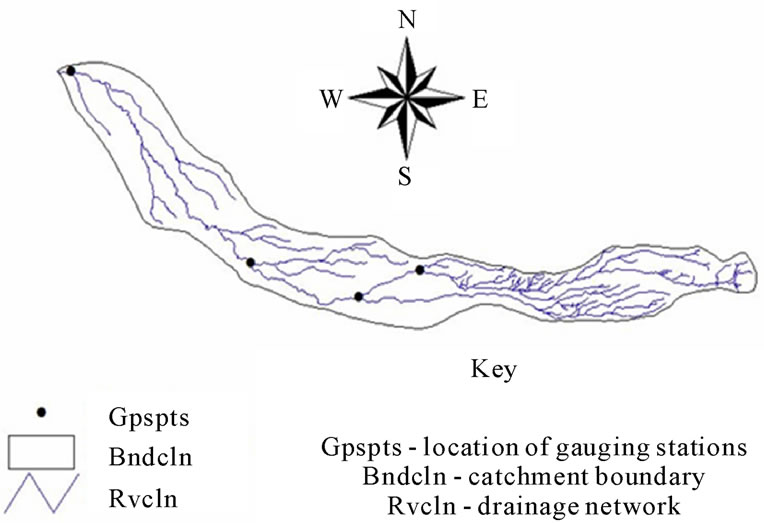
Figure 1. Drainage network and gauging stations in the Naro Moru catchment.
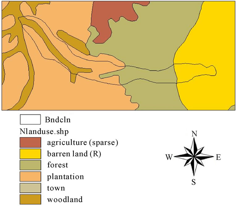
Figure 2. Land use types covering the study area.
range of applications for reasons that include its computational efficiency and flexibility on input data requirements [9]. The available data for the catchment under study could be used in hydrological modeling using SWAT. SWAT is capable of modeling changes in land use and management practices, can model variety of catchment areas ranging from a few hectares to thousands of square kilometers and performs long term simulations. Besides, the model is freely available and can be downloaded from the internet. The model website has a well developed system for support to model users. The model is in the public domain and therefore available without many restrictions. The model has options for daily, monthly and yearly time step simulations that can be carried out without altering the input data. Model predictions are spatially distributed thereby providing spatial information regarding upstream sources of modeled quantities [10].
2.3. The SWAT Model Review
2.3.1. Brief Description of the SWAT Model
SWAT model is a process based, continuous physically based distributed parameter river basin model that simulates water, sediment and pollutant yields developed in the early 1990’s to assist water resources managers asses impact of land use management on water, and diffuse pollution for large ungauged catchments with different soil types, land use and management practices [11]. Model components include weather, hydrology, erosion, soil temperature, plant growth, nutrients pesticides, land management, channel and reservoir routing [12]. The first step in creating a SWAT model involves delineation of the sub-watersheds in the basin each of which is treated as an individual unit. The sub basins are further divided into hydrologic response units (HRU’s). These units are composed of homogeneous land use, soil characteristics and management practices. Relevant hydrologic components like surface runoff, ground water flow and sediment yield are estimated for each HRU’s unit. Two methods are used for surface runoff estimation in SWAT i.e. the SCS curve number and Green-Ampt infiltration. This study is based on the use of curve number for surface runoff and hence stream flow simulation. A SWAT model can be built using the Arc-View interface called AVSWAT which provides suitable means to enter data into the SWAT code.
2.3.2. Swat Model Origin and Applications
The historical development and applications of the SWAT model is well documented in [13] in which it is reported that early origins of SWAT is traced to models previously developed by the United States Department of Agriculture, Agricultural Research Service (USDA-ARS) models that included the Chemicals, Runoff and Erosion from Agricultural Management Systems (CREAMS) model, Ground Water Loading Effects on Agricultural Management Systems (GLEAMS) model and the Environmental Impact Policy Climate (EPIC) model originally called Erosion Productivity Impact Calculator. The authors further note that the current SWAT model evolved from the Simulator for Water Resources in Rural Basins (SWRRB) model whose development commenced in the early 1980’s and through modifications that incorporated inputs from other models, the SWAT model finally developed when SWRRB was eventually merged with Routing Outputs Outlet (ROTO) model to overcome their limitations. Since its creation in the early 1990’s, the model has undergone continuous review and expansion of its capabilities.
The model has been applied worldwide for purposes that include simulation of sediment flow [14], modeling hydrologic balance [15], Evaluation of the impact of land use and land cover changes on the hydrology of catchments [16]. It has also been used to assess the effect of certain interventions on river and sediment flows [17]. The model has registered good performance as well as limited success. Limited success has been reported in SWAT simulation for stream flow in South African catchments [18]. Over estimation of flows between 1 and 3 mm was reported while flows between 4 and 7 mm were overestimated. The model performance was notably better in the dry than in the wet years. Discrepancies between the observed and predicted flow for the two catchments considered was attributed to their small drainage basins. The model was developed to simulate large catchments, a limitation which may affect model performance.
2.4. Model Evaluation
Graphical and statistical techniques were used for evaluating model performance. One of the evaluation statistics used was the Nash-Sutcliffe efficieny (NSE) being the most widely used evaluation criterion for testing the goodness of fit between the observed and simulated values. It indicates how well the plots of observed and simulated data fits the 1:1 line. The Pearson’s correlation coefficient (r) and coefficient of determination (R2) is another goodness of fit criterion used in this model evaluation to describe the degree of collinearity between simulated and observed data. The deviation of volume (DV) was also used in the model evaluation to asses over estimation or underestimation of the streamflow.
2.5. Data Preparation for Hydrological Modelling Using SWAT
2.5.1. Summary of Model Input Data
The input parameters required to run the model included;
• Daily precipitation
• Digital elevation Model (DEM)
• Weather data (e.g. solar radiation, wind speed, maximum and minimum temperature, and relative humidity).
• Soils information.
• Land use data.
• Drainage data
Digital elevation model (DEM)
DEM was created from contours and converted to a shape file covering the area under study. Figure 3 shows the DEM derived from the contours.
Land use input data preparation
The shape file land use map was compiled from the Kenya Soil Survey. These land use types were re-classi-
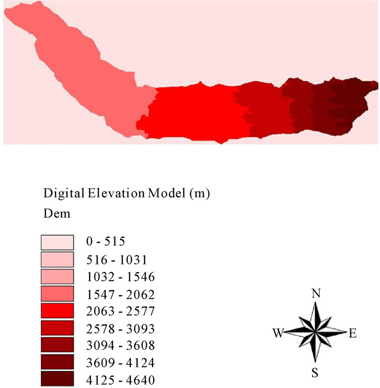
Figure 3. Digital elevation model (DEM) derived from contour network.
fied to the corresponding SWAT land uses for the model to load data. The land uses and abbreviations are shown in Table 1.
Soils input data preparation
Data for soil included the shape file soil map extracted from the soil map of Kenya available from Kenya Soil Survey (KSS). For each of the soil units in the study area, the soil physical and chemical properties were determined from the corresponding soil unit identified from the table of the soil properties (KENSOTER table). These properties included the proportions of sand, silt, clay and coarse fragments (i.e. % sand, % clay, % silt), bulk density (BD), Cation Exchange Capacity (CEC), Electrical conductivity (ELCO), Total Carbon (TOTC), etc. Some soil properties are shown in Table 2. Figure 4 shows the major soil units in the area. The use of KENSOTER soils data base to estimate the soil properties is well documented in [19].
Weather data input preparation
The location of the meteorological station with the weather data based on its UTM co-ordinates and elevation was required. The X-cordinate (Easting) and Y-cordinate (Northing) based on the Universal Transfer Mercator (UTM) co-ordinate system for the Nyeri meteorological station which was chosen to provide weather input data were 273695 and 992078 respectively. The station elevation was 1817 m above sea level.
The weather input variables required included; Solar radiation, wind speed, relative humidity, precipitation, dew point temperature, minimum and maximum temperatures. Based on the data available at the Kenya Me-
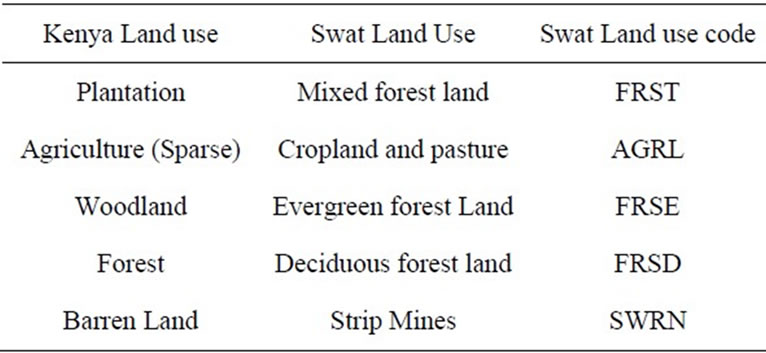
Table 1. Reclassification of observed land uses to SWAT land-use types.
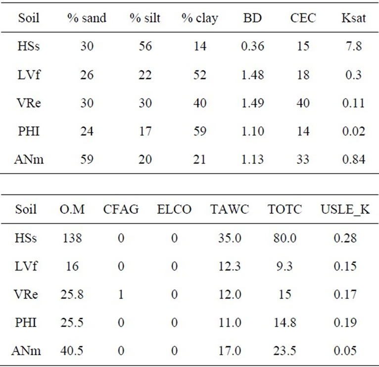
Table 2. Soil properties for soil units in the study catchment.
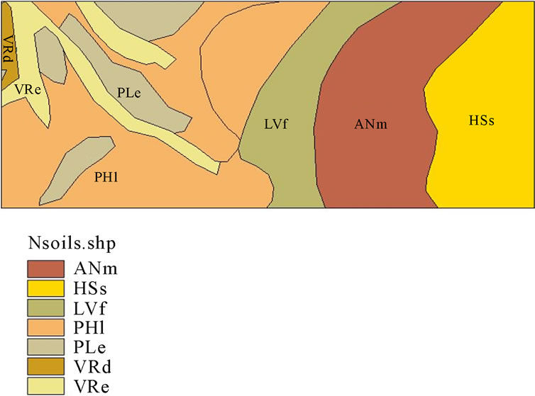
Figure 4. Major soil units in the study area.
teorological Station, it was possible to acquire the data for all the above weather variables for 9 years daily data during the period 1992-2000 based on three rainfall stations in the vicinity of the study catchment.
The weather generator
The weather generator provides input data to SWAT being statistical parameters derived from the weather information. The weather generator data was derived from the nine years daily data (1992-2000) on rainfall, minimum temperature, maximum temperature, relative humidity, wind speed, solar radiation and dewpoint temperature. The data output included the following for precipitation:
• Average monthly precipitation (PCP_MM).
• Standard deviation for precipitation (PCPSTD).
• Skew coefficient (PCPSKW).
• Probability of a wet day following a dry day (PR_ W1).
• Probability of a wet day following a wet day (PR_ W2)
• Average number of days of precipitation in month (PCPD).
Similar information was also determined for other weather variables. The above indicated model weather input data was determined using a programme known as pcpSTAT based on the daily weather data.
Drainage Data
Drainage data input into SWAT was provided in the form of digitized stream network. The digitized stream network was made available as shape file. The stream network used as input to SWAT together with the DEM was used in the catchment delineation using a selected watershed outlet.
2.5.2. Model Simulation Run
Having successfully loaded the indicated data, the model was able to run and produce the necessary output information on streamflow on a daily, monthly or yearly basis.
3. Results and Discussion
3.1. Preliminary Assessment of Model Performance
3.1.1. Daily Simulations
The model was initially run for a warm period of six months in which a daily simulation was carried out during the period 1/1/1992 to 30/6/1992. Daily and monthly stream flow simulations were then performed in the period 1/7/1992 to 30/6/1995 representing three years. Model evaluation was begun with simulation based on a daily time step. Figure 5 show the trend of stream flow hydrographs for the observed and simulated flows (m3/s) during the three year period based on the first modeling run.
The model over predicted flow during certain periods
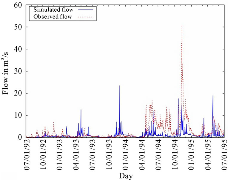
Figure 5. Hydrographs of observed and simulated daily flows during the period 1/7/92-30/6/95.
and under predicted in others while in some periods, the observed and simulated flows were in agreement. In general, the model under predicted high flows while simulating low flows fairly.
Comparisons based on daily time step are likely to be misleading due to the manner in which the model computes the daily flows which differs from that used in recording observed flows and this affects the values of peak flows. The observed flows are based on instantaneous readings taken at a certain time of day (e.g 9.00 am) in the morning while the simulated flows are based on the daily average. If heavy rainfall occurs close to the time when the observation is about to be read say 7 am in the morning the resulting peak flow is likely to be reflected in the observed record. However if the rainfall occurs much earlier e.g. the previous day, then it’s is likely that the resulting runoff will have passed the catchment outlet before a reading is taken so the peak flow would not be reflected in the daily flow reading. The surface runoff may, however, be captured by the flow simulation especially if the daily flow is reasonably high so that the daily average of the runoff will have a high value. For storm events that occur closer to the time of observation, the peak flows are captured by both the observed and simulated flows. Figure 6 shows a comparison of observed and simulated flows based on linear regression with values of the y-intercept and coefficient of determination (R2) also indicated.
The value of R2 was found to be 0.144 while NashSutcliffe efficiency (NSE) 0.01 relecting a poor linear relationship between the observed and predicted values based on daily simulation. This poor performance, which is often misleading, may be attributed to small differences in the timing of observed and simulated hydrographs likely to occur when using daily rainfall data. Daily
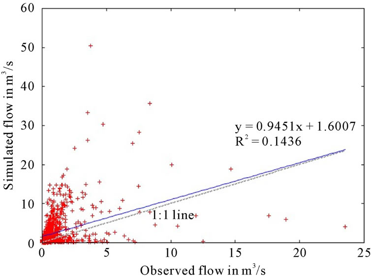
Figure 6. A Comparison of simulated and observed daily flow during the period 1/7/92-30/6/95.
simulations do not provide values that are expected to compare reasonably well with the predicted ones. This is partly due to the poor prediction procedure for peak flows. As a result therefore, detailed evaluation of the model performance including model calibration was done based on monthy time step. This is in consideration of the fact that monthly values are likely to be more representative than the daily values since with daily values cummulated over the month, the daily errors are likely to be cancelled out. Hence the subsequent calibration process was considered on the basis of monthly simulations.
3.1.2. Monthly Simulations
Simulation was done based on monthly basis to observe the perfomance of the model based on a montly time step. Figure 7 shows the hydrographs of the average daily flows for each month for observed and predicted flows during the period 1/7/92 to 30/6/95 during the first modelling run. From the figure, it can be observed that the model performance has improved compared to that based on a daily time step.
A Similar observation was made by [20] while evaluating performance of SWAT model in the Nzoia catchment in western Kenya in which the author noted that the agreement between observed and simulated flows was stronger with monthly than with daily flows during calibration. During the period July 1992 to around April 1994, the model predictions of stream flow seem to agree with the observed values except for a few instances where there was over prediction of flow like in December 1994. For the period April 1994 to June 1995, the model generally under predicted the flows. The model is a therefore a poor simulator of high flows but fairly simulates low flows. Figure 8 shows a plot of observed and predicted flows based on the linear regression. The values of the coefficient of determination and regression
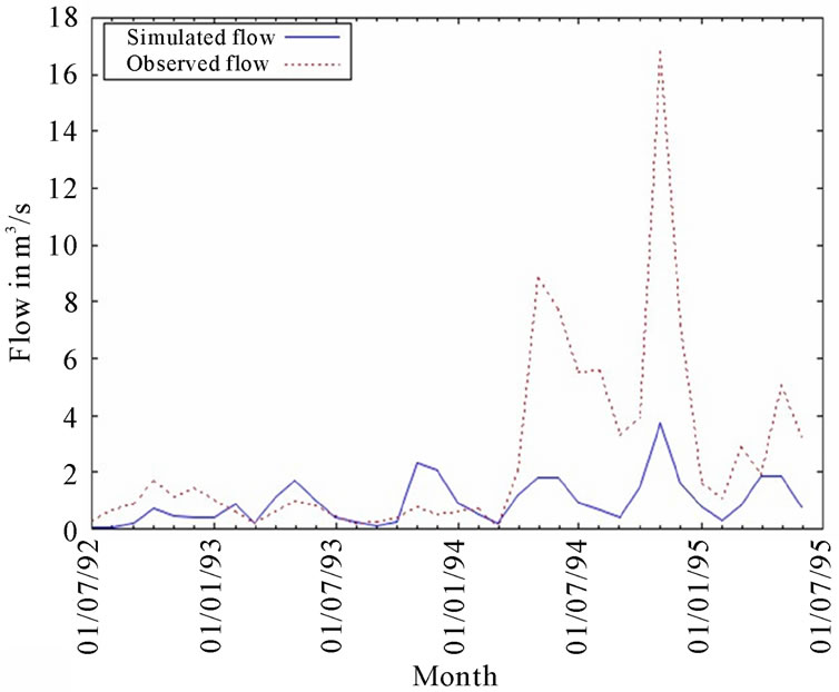
Figure 7. Hydrographs of simulated and observed mean daily flows in month for the period July 1992 to June 1995.
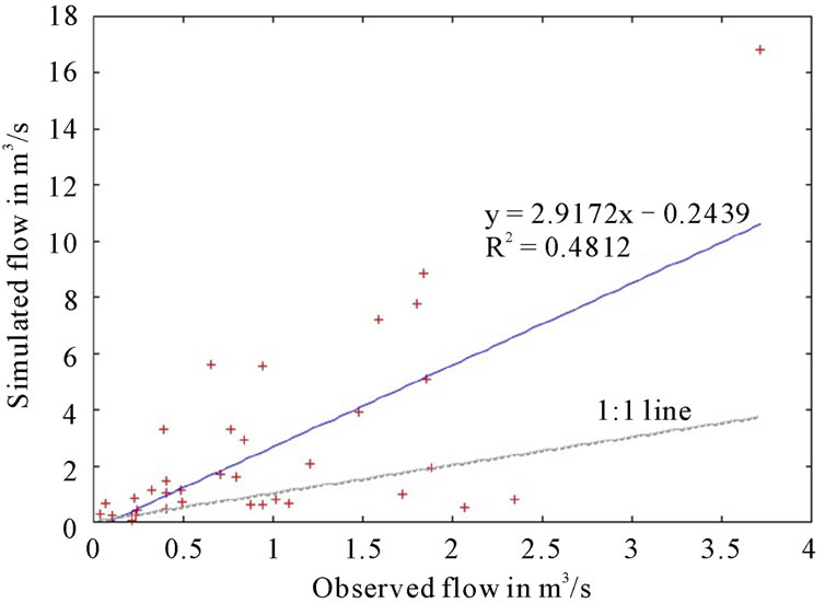
Figure 8. Comparison of observed and predicted mean daily flows in the month for the period 1/7/1992 to 30/6/1995.
equation expressing the linear relationship are as well indicated.
The value of the coefficient of determination (R2) of about 0.5 indicates acceptable performance. The correlation coefficient r = 0.7 showing that the predicted and observed flows exhibit linear relationship. The NashSutcliffe efficiency, however registered a low value of 5% indicating poor simulation performance. The low value of NSE can be attributed to a strong deviation volume (Dv) of 61.7% as noted by [11]. The high positive value of Dv indicates the average tendency of the simulated flows to under estimate the flows. The process of model calibration was carried out to further assess model performance and to examine possibilities of domesticating the model for application in the local catchment.
3.2. Sensitivity Analysis and Model Calibration
Sensitivity analysis was carried out to find the order of sensitivity of stream flow to the input parameters. The sensitivity analysis process was carried out automatically by the model. The model produced the output indicating the order of sensitivity of the model input parameters. Table 3 shows an extract of the summary of the output format from sensitivity analysis. Interpretation of the results indicate that the curve number (CN2) is the most sensitive parameter. The ranking of the parameters is indicated in the row labeled “out”.
An auto calibration process was the carried out based on a selection of the three most sensitive parameters. These were the Curve number (CN2), Soil Evaporation compensation factor (ESCO), and the Threshold water depth in the shallow aquifer for “revap” (QWQMN). After the auto calibration process, the best values of the selected parameters for which the model prediction closely agreed with the observed were determined and produced in the auto calibration results.
The model was again rerun based on these values. Not much change was noted in the hydrographs of observed and simulated flows after the auto calibration process. A comparison of observed and predicted monthly flows yield a coefficient of determination slightly above 0.50 with minimal change in the value of NSE which still remained low at 6% and a small reduction in deviation volume to 61.3%. This indicated acceptable but modest performance of the model for the catchment in question. An attempt was made to perform a manual calibration of the model. This was done by varying each of the three most sensitive parameters by 10% from their default values, but within the allowable range, and selecting the value that provides the best possible agreement between observed and simulated flows. The parameters were varied one at a time while keeping the others constant until an optimal value is obtained. A slight, but insignificant improvement was observed in the values of the evaluation statistics with r = 0.72 (R2 = 0.51) and NSE of 5%, with the deviation volume rising to 64%. Table 4 shows the calibration results. The seemingly poor performance performance of the model could be associated with input data deficiencies also observed by [21]. Daily rainfall data in the vicinity of the catchment was available from three rainfall stations in which only two were located within the catchment and near the outlet. The third station was located outside the catchment near the upstream end. Hence the rainfall may not have been representative. Only one full meteorological station was available with adequate weather data for use in the modeling but was located well outside the catchment. The weather data may therefore, also not have been adequately representa-
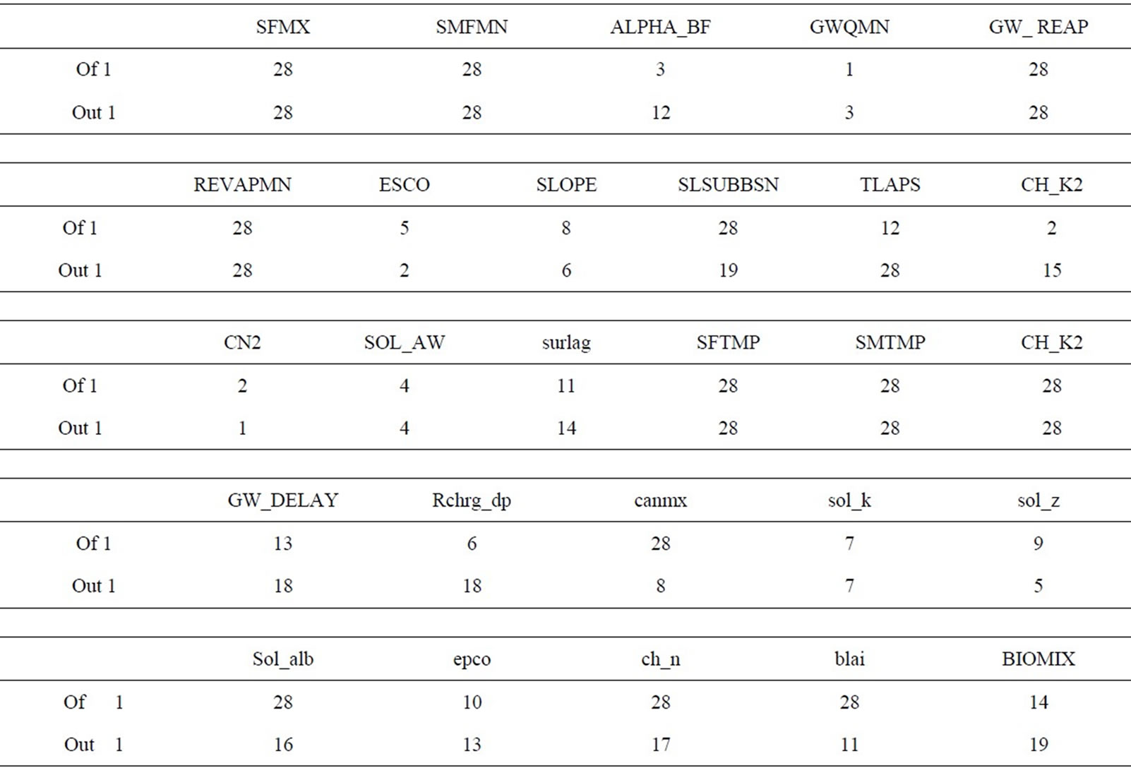
Table 3. Sensitivity analysis results showing the order of sensitivity of input parameters.

Table 4. Evaluation of model results for first simulation runs, calibration and validation.
tive. Besides, there were also cases of missing data during certain periods for thestations used.
3.3. Model Validation
Based on the optimized parameters obtained during the calibration period, a further simulation was carried out to assess the model performance during the period 1/1/98 to 31/12/2000 which is outside the period when the model was calibrated. Figure 9 shows the graphical representation of the observed and simulated flows during this validation period. The hydrographs of stream flow during the period of validation show that the simulated and observed flows show a nearly close fit, an indication of improved model performance.
Figure 10 shows a plot of simulated against observed monthly flows.
There is evidently improved performance of the model with the coefficient of determination, R2 = 0.58 (r = 0.76). The NSE value significantly improved to 0.51 while the deviation volume reduced to 24.7%. This reflects acceptable model performance [22] which is can be considered satisfactory and therefore promising for applicability in the catchment. A summary of calibration and validation results are indicated in Table 4.
3.4. General Assesment of Model Performance
The results obtained in this study are not unique. Applications of SWAT worldwide has yielded diverse results
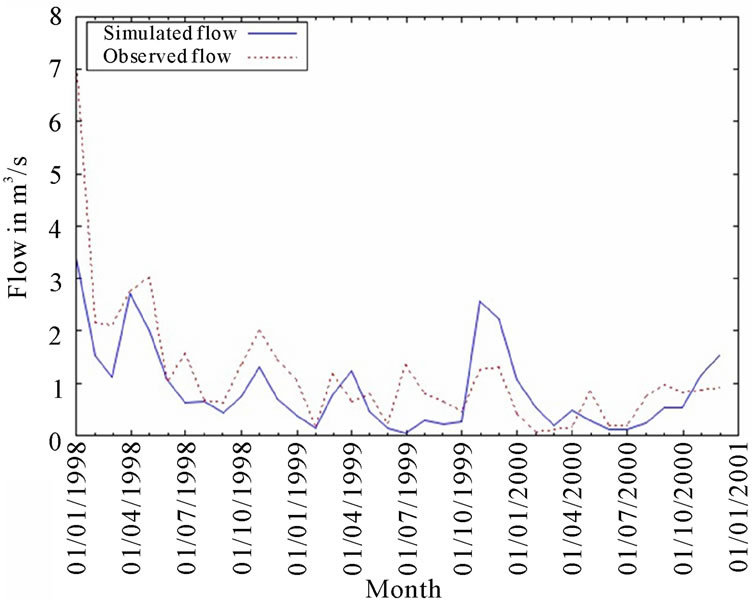
Figure 9. Hydrographs of simulated and observed mean daily flows in month for the validation period 1/1/98 to 31/12/2000.
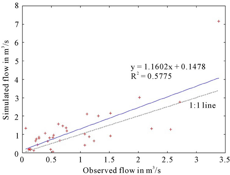
Figure 10. Comparison of observed and predicted mean daily flows in the month for the period 1/1/1998 to 31/12/ 2000.
some encouraging while in some instances, the success in the use of the model has been limited. This may be attributed to strengths and weaknesses associated with the use of SWAT across the world spectrum. A few studies involving SWAT supports this observation. Good model performance has been reported by [23] while modelling water balance with SWAT on three catchment areas in northern Germany. However, the first model runs failed to represent the streamflow correctly (also observed in this study) showing underestimation of observed high winter discharge peak and over estimation of baseflow. Success in model prediction was attributed to repeated attempts to improve the model performance. The challenges of modeling with SWAT in lowland areas are mentioned and which had to be taken into account in model parameterization. [9] evaluated the performance of the SWAT model in several sub basins in Chile. The model performance was not uniform in all the sub catchments studied. The NSE index ranged from good to satisfactory for the calibration period depending on the sub basin. The model was observed to have under estimated peak flows, a similar observation to this study. An explanation for this was given as inadequate description of rainfall input field due to the limited number of available meteorological stations and poor representation in higher areas due to orographic effects. This scenario is similar to this study. Only one rainfall station was available to represent the rainfall near the higher elevations of Naro Moru catchment. The station was also outside of the catchment but was the nearest available for use. The standard interpolation method used in AVSWAT for estimating rainfall (Thiesen polygons) was notably a limitation as its reliability is yet to be tested if discrete improvements in model performance is to be expected.
4. Conclusion and Recommendations
The model predictions of streamflow based on monthly simulations compared fairly well with the observations in the preliminary assessment and even after calibration yielding a coefficient of determination (R2) of about 0.50 reflecting acceptable performance. Better results were obtained during the validation period yielding a value of R2 ≈ 0.6, NSE = 0.51, and Deviation Volume (Dv) of 24.7%. This indicated satisfactory performance of the model. Modest model performance was attributed to input data deficiencies partly associated with unrepresentative rainfall input data. Better results can be obtained through the use of more detailed, complete and more accurate data. Preliminary model assessment based of ordinary simulation and auto calibration does not give a adequate evaluation of model performance, however it gives an indication on the possibility of model applicability for local conditions. Improved simulations can be achieved by the use of better and more detailed data and better parameter calibration efforts.
5. Acknowledgements
I wish to acknowledge the support of the University of Nairobi in funding the research through the Dean’s committee research grant. I wish to thank all the institutions that assisted in the provision of data used in the study including Kenya Soil Survey (KSS), Ministries of Lands and Settlement and of Water and Irrigation, Kenya, Kenya Meteorological Department, and the Natural Resource Monitoring, Management and Modelling (NRM3), Nanyuki, Kenya. I also wish to acknowledge the useful comments and contributions from the anonymous reviewers that played a key role in improving the manuscript.
REFERENCES
- E. G. Bekele and H. V. Knapp, “Hydrologic Modeling of Fox Watershed: Model Development, Calibration, and Validation,” Proceedings of the World Environmental and Water Resources Congress, Honolulu, Hawaii, 12-15 May 2008, pp. 1-10. doi:10.1061/40976(316)588
- S. K. Jain, and K. P. Sudheer, “Fitting of Hydrologic Models: A Close Look at the Nash-Sutcliffe Index,” Journal of Hydrologic Engineering, Vol. 13, No. 10, 2008, pp. 981-986. doi:10.1061/(ASCE)1084-0699(2008)13:10(981)
- B. Schmalz, F. Tavares and N. Fohrer, “Modeling Hydrological Processes in Mesoscale Lowland River Basins with SWAT-Capabilities and Challenges,” Hydrological Sciences Journal, Vol. 53, No. 5, 2008, pp. 989-1000. doi:10.1623/hysj.53.5.989
- S. N. Ngigi, “Hydrological Impacts of Land Use Changes on Water Resources Management and Socio-Economic Development of Upper Ewaso Ng’iro River Basin in Kenya,” PhD Thesis, Delft University of Technology, Netherlands, 2006.
- M. K. Thomas, H. P. Liniger and F. N. Gichuki, “Development of a Stream flow Model for Rural Catchments in Kenya,” Proceedings of the Fourth National Workshop on Land and Water Management in Kenya: Towards Sustainable Land Use, Kikuyu, Kenya, 15-19 February 1993, pp. 191-202.
- J. M. Gathenya, H. P. Liniger and F. N. Gichuki, “Problems of River-Water Management for a Basin West of Mount Kenya: Challenge to Water Resource Planners,” Proceedings of the Fourth National Workshop on Land and Water Management in Kenya: Towards Sustainable Land Use, Kikuyu, Kenya, 15-19 February, 1993, pp 175-180.
- S. L. Neistsch, J. G. Arnold, J. R. Kiniry and J. R. Williams, “Soil Water Assessment Tool Theoretical Documentation (Version 2005),” Grassland Soil and Water Research Laboratory, Temple, Texas, 2005, pp. 1-27.
- P. M. Ndomba and B. Z. Birhanu, “Problems and Prospects of SWAT Model Applications in NILOTIC Catchments: A Review,” Nile Water Engineering Scientific Magazine, Vol. 1, 2008, pp. 41-52.
- A. Stehr, A. P. Debeles, F. Romero and H. Alcayaga, “Hydrological Modeling with SWAT under Conditions of Limited Data Availability: Evaluation of Results from Chilean Case Study,” Hydrological Sciences Journal, Vol. 53, No. 5, 2008, pp. 588-601. doi:10.1623/hysj.53.3.588
- G. Andualem and M. Yonas, “Prediction of Sediment Inflow to Legedadi Reservoir Using SWAT Watershed and CCHELD Sediment Transport Models,” Nile Basin Water Engineering Scientific Magazine, Vol. 1, 2008, pp. 66-74.
- E. Levesque, F. Anctil and A. Van Griensven, “Evaluation of the Streamflow Simulation by SWAT Model for Two Small Watersheds under Snowmelt and Rainfall,” Hydrological Sciences Journal, Vol. 53, No. 5, 2008, pp. 961-976. doi:10.1623/hysj.53.5.961
- R. Rostamian, A. Jaleh, M. Afyuni, S. F. Mousavi, M. Heidarpour, A. Jalalian and K. C. Abbaspour, “Application of a SWAT Model for Estimating Runoff and Sediment in Two Mountaneous Basins in Central Iran,” Hydrological Sciences Journal, Vol. 53 No. 5, 2008, pp. 977-988.
- P. W. Gassman, M. R. Reyes, C. H. Green and J. G. Arnold, “The Soil Water Assessment Tool: Historical Development, Applications and Future Research Directions,” Transactions of the ASABE, Vol. 5, No. 4, 2007, pp. 1211-1250.
- P. M. Ndomba, “Modelling of Sediment Upstream of Nyumba Ya Mungu Reservoir in Pangani River Basin,” Nile Basin Water Science & Engineering Journal, Vol. 3, No. 2, 2010, pp. 25-38.
- S. G. Setegen, R. Srinivasan and Bijan Dargahi, “Hydrological Modelling in Lake Tana Basin, Ethiopia Using SWAT Model,” The Open Hydrology Journal, Vol. 2, 2008, pp. 49-62.
- P. M. A. Odira, M. O. Nyadawa, B. Okello, N. A. Juma and J. P. O. Obiero, “Impact of Land Use/Cover Dynamics on Stream Flow: A Case Study of Nzoia River Catchment, Kenya,” Nile Water Science and Engineering Journal, Vol. 3, No. 2. 2010, pp. 64-78.
- M. P. Tripathi, R. K. Panda and N. S. Raghuwanshi, “Development of Effective Management Plan for Critical Sub Watersheds using SWAT Model,” Hydrological Process., Vol. 19, No. 3, 2005, pp. 809-826.
- M. Govender and C.S. Everson, “Modelling Streamflow from Two Small African Experimental Catchments Using SWAT Model,” Hyrological Processing, Vol. 19, No. 3, 2005, pp. 683-692.
- N. H. Bartes and P. Gicheru, “Soil Data Derived from SOTER for Studies of Carbon Stocks and Change in KENYA (Version 1.0),” Project Report 2004/01, ISRIC-World Soil Information, 2004.
- F. Githui, F. Mutua and W. Bauwens, “Estimating Impacts of Land Cover Change on Runoff using the Soil water Assessment Tool (SWAT): Case Study of Nzoia Catchment, Kenya,” Hydrological Sciences Journal, Vol. 54, No. 5, 2009, pp. 899-908. doi:10.1623/hysj.54.5.899
- R. Jayakrishnan, R. Srinivasan, C. Santhi and J. G. Arnold, “Advances in the Application of the SWAT Model for Water Resources Management,” Hydrolocal Process, Vol. 19, No. 3, 2005, pp. 749-762.
- D. N. Moriasi, J. G. Arnold, M. W. Van Liew, R. L. Binger, R. D Harmel and T. L. Veith, “Model Evaluation Guidelines for Systematic Quantification of Accuracy in Watershed Simulations,” Transactions of the American Society of Agricultural and Biological Engineers (ASABE), Vol. 50, No. 3, 2007, pp. 885-900.
- B. Schmalz, F. Tavares and N. Fohrer, “Modelling Hydrological Processes in Mesoscale Lowland River Basins with SWAT-Capabilities and Challenges,” Hydrological Sciences Journal, Vol. 53, No. 5, 2008, pp. 989-1000. doi:10.1623/hysj.53.5.989

