Journal of Software Engineering and Applications
Vol.11 No.06(2018), Article ID:85733,23 pages
10.4236/jsea.2018.116020
Matching Source Code Using Abstract Syntax Trees in Version Control Systems
Jonathan van den Berg, Hirohide Haga
Graduate School of Science and Engineering, Doshisha University, Kyoto, Japan

Copyright © 2018 by authors and Scientific Research Publishing Inc.
This work is licensed under the Creative Commons Attribution International License (CC BY 4.0).
http://creativecommons.org/licenses/by/4.0/


Received: May 29, 2018; Accepted: June 26, 2018; Published: June 29, 2018
ABSTRACT
Software projects are becoming larger and more complicated. Managing those projects is based on several software development methodologies. One of those methodologies is software version control, which is used in the majority of worldwide software projects. Although existing version control systems provide sufficient functionality in many situations, they are lacking in terms of semantics and structure for source code. It is commonly believed that improving software version control can contribute substantially to the development of software. We present a solution that considers a structural model for matching source code that can be used in version control.
Keywords:
Version Control, Source Code Matching, Abstract Syntax Tree, Structured Representation

1. Introduction
Version control systems are one of the most important tools in software engineering. They are used to manage software projects that can consist of millions of lines of code, and shared by hundreds of colleagues that all work on the same software project. A version control system is the bridge between these colleagues and allows them to work efficiently in the same computer documents simultaneously. Nearly each and every software project where multiple people collaborate to develop software uses such a version control system. Without version control systems, the world would not have reached its current state as software development would have proven to be a lot more difficult.
However, version control systems still have a lot of points for improvement. Many problems still occur while using a version control system as its fundamentals are flawed. Bryan O’Sullivan wrote the article “Making sense of revision-control systems” in September 2009 [1] and stated that:
Much work could be done on version control systems’ formal foundations, which could lead to more powerful and safer ways for developers to work together.
This article is a research result that proposes one possible solution for such a more powerful and safer version control system. This solution is inspired by the research on version control systems conducted by Wouter Swierstra [2] , who has recently written the article “The Semantics of Version Control’’ [3] in 2014. In his article he brings up several logical and mathematical solutions [4] to reason about the state of a version control system. And does so by defining a semantics and thus, laying a formal foundation.
Even though a formal foundation has been laid, the current solution still seems to be flawed and can be further improved. This solution consists of a mathematical approach that defines a semantics and while its approach does allow us to reason about the state of a version control system, it does not truly understand its contents. This has motivated us to come up with a better approach that gives such insight to file contents. The contents of a software project mainly consist of source code files, which are simple line-based text files containing the source code of a software application. These lines of text contain instructions for the computer to execute and are modeled after the chosen programming language for the application. Therefore, they contain a certain structure and have a syntax and a semantics so that the language can be reasoned about. The solution we present is to utilize the structure and syntax of programming languages in order to be able to reason about the semantics of a version control system and is based upon “A 3-way merging algorithm for synchronizing ordered trees: the 3DM merging and differencing tool for XML’’ [5] by Tancred Lindholm. In the next few sections, we will show how it is related to our solution for improving version control systems. Since then, however, no further essential advancement was found in literatures. This is partly because of the less understanding of the importance of theoretical background of version control systems. Version control systems are widely used now and further advancement requires the theoretical and semantical basis of them. Therefore, we try to establish the more formal and theoretical basis of version control. By using our proposed basis, advanced functions will be able to implement.
2. Problem Description
2.1. General Description
In this article, we will address how the structuring, matching and merging can be improved over existing methods from an algorithmic point of view. When we consider structuring, matching and merging, we will face certain problems that many existing version control systems out there have been confronted with as well:
• How can we convert source code into structured data?
• How do we determine which parts they have in common in the structured data?
• How can the structured data be merged both precisely and efficiently?
In addition, the algorithm that serves as a solution to the above stated problems also faces certain requirements, with the most important requirements being:
• Generalizable and applicable to multiple programming languages instead of a single specific programming language.
• Well defined, a formal definition must be laid such that it can be reasoned about and by all means undefined behavior should be avoided or even impossible.
• No locking mechanisms can be involved; it should be possible to have multiple branched files of a certain base file for optimal collaboration possibilities.
• Deterministic, such that no randomness is involved and thus will always produce the same output given some input or initial state.
Of course, there are other requirements as well, such as file management, but we will consider those as basic version control system requirements and will therefore not be discussed in this article. Conforming to all these requirements is part of the challenge to design an algorithm that solves the previously mentioned problems as well. Our approach regarding how we will meet these requirements will be explained when we present the solution algorithm.
2.2. Converting Source Code into Structured Data
The approach used in popular version control systems is a line-based approach. They divide a source code file in lines and structuring them in a linear manner, such as a linked list or array. Given the fact that this method can be generalized and used on any text-based file, it implies that it is a good method for merging source code files as well. This answers the first problem regarding designing a version control system in a simple way, but leads to issues when we face the second problem. If we have to determine which parts two files have in common, it will prove to be difficult as we have to check each line against another. Even if we would consider this an efficient way, further difficulties will appear when there are two simultaneous edits on the same line. In such a case there would be a conflict, and it has to be resolved by either character by character merging or manual conflict resolving as it does not truly understand the underlying structure. It is commonly believed that general structural differencing problems cannot be reduced to linear differencing problems [6] . In other words, we have to provide a non-linear data structure that truly represents a source code file contents.
2.3. Matching Common Parts in the Structured Data
The next problem we face is determining which parts two files have in common in the structured data. If we want to change the structured data that represents a source file, then we have to change the algorithm that can detect parts that two source files have in common, referred to as the matching algorithm from now on. Ideally, we want to match as many parts as possible since it will save us the effort in the merging stage. Although we will have a changed data structure, a fundamental way of comparing should be obvious; string comparison. Since we are dealing with plain text files, string comparison is almost unavoidable, just like it is in existing version control systems. However, in the later section, we will propose several other methods that can be used for the matching algorithm as well.
3. Merging the Structured Data Precisely and Efficiently
Each time we want to merge two files, a so called conflict may occur. It means that the version control system failed to merge the code and cannot proceed. These conflicts have to be resolved by a developer and cannot be done automatically. The correct source code has to be handpicked by the developer and this has proven to be an annoying issue in the world of software engineering. Resolving a conflict consumes time and slows down the development of the software. In order to avoid conflicts, we should consider a precise but also efficient algorithm based upon the matching algorithm. Part of this merging algorithm is detecting where operations such as inserting, deleting and possibly also replacing, moving and renaming find place [2] .
Requirements for Matching and Merging
When a solution is provided, it also has to meet certain requirements. The first and most important requirement it that it should be generalizable and applicable to multiple programming languages. Being limited to a relatively small scope is what we want to avoid, which is why we want it to be generalizable, much like the common line-based approach. In order to be able to reason about, a well defined and formation definition should be provided such that undefined behavior can be avoided. In addition, the behavior of the algorithm should be predictable in accordance with the definition, in such a way that developers are not surprised when a conflict occurs. Although it is obvious in any modern version control system, users should be able to work on the same file simultaneously. Therefore, no locking mechanisms that restrict access to a certain file can be involved such as in the case of the Source Code Control System (SCCS) [7] . In fact, if such a locking mechanism were to be involved, it would be completely unnecessary to provide a matching and merging algorithm in the first place. The final major requirement is that the solution must be deterministic. No randomness can be involved in the algorithm in such a way that a certain input always gives the same output. In accordance to the second requirement specified, the behavior should be well defined and predictable. No chances should be taken in the matching algorithm, if we match two parts we need to be sure that they are indeed the same. For the merging algorithm, operations should be detected in a deterministic manner as well. The above requirements provide the fundamental basis of our algorithm as we should comply to them before considering a solution that solves the problems mentioned in previous sections. We will provided it exactly in next section.
4. Solution and Implementation
Throughout this section, we will provide the solution to the problem statement described before. The semantics of current version control systems are lackluster and should be redesigned in order to improve version control systems. As Wouter Swierstra mentioned in his article “The Semantics of Version Control’’ [2] :
Version control systems manage the access to a (shared) mutable state. Therefore, they should be designed using a logic for reasoning about such a state.
He presents an approach where he sees a source code file as a sequence of lines of text, which can be operated on by mathematical functions. This approach allows us to reason about the mutable state of a version control system. Although this allows us to reason about version control systems, it does not allow us to reason about the true content of a source code file. Instead of a line-based solution, we will present a solution with a syntax-based approach.
4.1. Using Abstract Syntax Trees as Internal Structure
The goal of our research is to merge source code by truly understanding its contents. One thing that all programming languages have in common is that they can be broken down into a so-called abstract syntax tree (AST), which is commonly used in compilers and interpreters as well. For example, Figure 1 is the data structure of a basic “if-statement’’:
Every programming language consists of a certain collection of syntax nodes and syntax tokens. Usually syntax nodes correspond to non-terminal symbols and syntax tokens correspond to terminal symbols. The scale of such a collection is language specific and therefore a formal model exists for each individual programming language. Syntax tokens are typically leaves in the AST as they are merely a token and cannot be divided in to smaller components such that they can have children as well. However, they can have so called syntax trivia, or layout characters, which are essentially pieces of text that do not represent any actual program code. Examples of trivia are white spaces, tabs, comments and so on. Trivia are excluded from the AST when they are used to compile source code

Figure 1. The structure of “if-statement”.
into an executable program, but for our case we should include them as we do not want comments and white space to be discarded from our algorithm output. Throughout this article, we will assume trivia to be included in their parent token as it reduces tree size and reduces time complexity.
Tokens and trivia cannot construct a tree and that is where syntax nodes come in. These do not represent any actual text content directly, but are composed of syntax tokens and other syntax nodes rather than strings. In order to be able to distinguish syntax nodes from each other they have a so called node kind, which as one may expect, indicates the kind of the node.
Def. 1 Let n be a node in any given tree T, and the set of all possible node kinds in a given programming language G, we denote the kind of n with the function .
An example of a node kind would be a method declaration or an if-instruction. Depending on the programming language, there may be very few to many kinds of nodes. How this kind attribute will play a role in the matching algorithm, will be made clear later in this section (Figure 2).
Although we have defined ASTs in a generic way above, it will quickly prove that using only text-based nodes and tokens is not a feasible solution as comparing text can be an expensive operation depending on the length of the text. Therefore, we should provide another property that does not depend on the input length, but only on the size of the AST in terms of nodes.
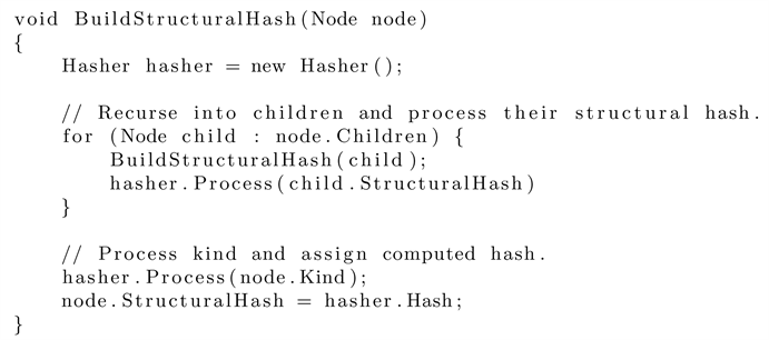
Hashing is a common method to determine equality between strings of large sizes efficiently in constant or linear complexity. In order to apply hashing to an AST, we have to apply hashing to every syntax token, syntax node and trivia in the tree. We want each node to have a unique hash value depending on its descendant nodes, such that we can determine equality between two hashed sub trees. An existing data structure has already been invented roughly forty years ago and is called a Merkle-tree, named after its inventor Ralph Merkle [8] . We construct a tree based on the concept of a Merkle-tree in a bottom-up fashion, where the leaves contain an initial hash value. The concept of this should sound familiar, as the structure of it fits perfectly with the AST structure where leaves are syntax tokens and all the ancestors are syntax nodes. Figure 3 is an example tree where the leaves can be considered as syntax tokens (including trivia) and its parents as syntax nodes:
Although the above example in Figure 3 shows a single hash value for each node in the tree, our solution uses two hash values that can be used for two

Figure 2. An AST represented by nodes, tokens and trivia.

Figure 3. An example of an a Merkle (hashed) tree.
kinds of equality between two nodes: a content hash and a structural hash. Both are computed in a similar manner, as we described earlier, by computing a node’s hash value based on its child nodes. However, there is a fundamental difference; in an AST, both nodes and tokens have a structural kind. Therefore, structural hashes can be calculated in a simple manner such as the pseudocode described below:
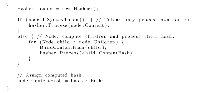
On the contrary, only the tokens in the tree have a content value, as the content of parent nodes is represented by the content of all descendant tokens in left-to-right order. Therefore, we have to calculate the content hash depending on whether it is a syntax token or not. Below is a similar but slightly altered version of the one shown above:
Using the two algorithms described above, we have a content hash and structural hash for each syntax node and syntax token in the AST. In further sections, it will become clear how we can utilize these hash values for an efficient matching algorithm.
4.2. Determining Common and Similar Structured Data
Typically, determining common and similar parts between two pieces of text does not prove to be a complicated process. However, these typical approaches do not consider any structure other than a sequence of characters which is why comparing characters is the only solution. In our case, we are dealing with a more complicated structure that consists of many aspects and components. Through out this section we will explain how we will utilize them in order to produce an accurate, yet efficient algorithm to measure similarity.
We mentioned the use of hashing to solve the performance issue of comparing large pieces of text, after having introduced use of hashing in an AST in the previous section, we will now define two measures of node similarity; content similarity and structural similarity. These similarity measures are used for the matching algorithm and utilize the content hash and structural hash, when we want to find a match for a certain node.
4.2.1. Measuring Content Similarity
Content similarity is defined by measuring similarity of the string content that is contained by a pair of nodes and . A simple method to measure string similarity between a pair of nodes is to perform a string similarity algorithm on their entire content string at once. However, this gives us little information about the amount of syntax tokens that were actually changed. In order to get more information regarding tokens, we have to traverse descendant tokens and compare the text they have in common instead. Which means they must be structurally similar as well to a certain degree, otherwise its not possible to know which syntax tokens to compare with each other. When comparing syntax tokens, similarity is typically expressed in characters, in which case long text tokens would be weighted heavier than short text tokens. This is something we want to avoid, tokens should be weighted equally as a short text token represents the same amount of information as a long text token. Therefore, for syntax nodes and syntax tokens we define a fixed base weight to which we refer to as node information weight. This weight may for example, differ depending on the kind of the node.
While tokens only have a base weight, syntax nodes also include the weight of their child nodes. In addition, we define content similarity based upon this information weight. The definitions for information weight and content similarity can be found below:
Def. 2 Let n be a node, we define the information weight for n as the base weight plus the sum of its children .
Def. 3 Let n and m be a pair of syntax tokens, we denote the token information weight for n and m with the function .
Def. 4 Let n and m be a pair of syntax tokens, we denote content similarity between n and m with , where is a normalized similarity algorithm such that .
The string similarity algorithm is undescribed thus far and can be any string distance algorithm that produces acceptable results. There are many existing string distance algorithms, such as the well-known “Levenshtein distance’’ and Longest Common Subsequence algorithms’’. Although these produce accurate results, we do not use the distance measure directly to measure the similarity between a pair of nodes. This is because we use the string distance as measure of certainty that one node really does match another, which we will explain in further detail later on. Therefore, the time complexity becomes important as long as the results of a given string similarity algorithm are acceptable. Which means that we can use an algorithm that approximates string similarity rather than precise string similarity.
The algorithm we use to measure string similarity is based on the “Q-gram algorithm’’ which was originally defined in “Approximate string matching with Q-grams and maximal matches’’ [9] . It was used instead of the more commonly used edit distance, such as Levenshtein distance and Longest Common Subsequence, due to running time complexity considerations. These edit distance algorithms run in , where d is the edit distance, whereas the Q-gram distance can be computed in :
Def. 5 Let be a finite set of elements (i.e. alphabet) and be all sequences of length q over . A Q-gram is a sequence .
Def. 6 Let v be a Q-gram and a finite sequence. If for some i, then v occurs in x. We denote the number of occurrences of v in x with the function and denote the similarity between two sequences x and y with: .
In our algorithm we decide the length of Q based on the minimum length of two sequences we want to compare, where the minimum length is denoted . For a minimum length of equal to or less than 20, Q is 2 and otherwise Q is the square root of :
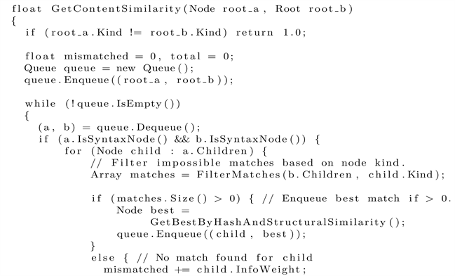
Based on the above definitions of the Q-gram algorithm, we have now defined the measure that can evaluate the content similarity between a pair of syntax tokens. The next step is to use the content similarity of tokens and propagate their values up the tree structure as we want to be able to compare syntax nodes as well. The concept behind content similarity between a pair of syntax nodes is that we take the sum of the weighted content similarity of all descendant syntax token pairs denoted , such that:
This means that we must perform a certain kind of tree traversal, as we need to construct the token pairs used in the above equation. Throughout this section, “pair of nodes” has been mentioned several times for a reason. As in our algorithm, we attempt to pair two nodes wherever it is possible, but without spending too much time looking for the best match. The initial pair should be straight-forward as it consists of the initial two input syntax nodes n and m such that and . While the next step is to select a match for all where is child node of n. The match is selected from m’s child nodes denoted . The method to select a child from m that fits some consists of two stages: filtering impossible matches and finding the best matching child node within possible matches. The first stage is based on the kind of a node, which we defined in previous section.
Def. 7 Let and be a pair of nodes, then and are an impossible match if where and are the node kinds of and , and G is a given programming language.
After filtering impossible matches and likely the majority of pairs, we should find the best match from the possible matches. Should there be no matches left, we then have a complete mismatch and content similarity of zero is assumed. If we have only one possible match, our next iteration is clear as similarity should be measured with the only possible match. However, in the case of multiple possible matches we have to determine which match likely fits the original node, referred to as the best match from here on.
We have to perform a matching procedure such that we compare the right nodes with each other. This matching procedure is based upon the hash algorithm explained previously and the structural similarity algorithm that we will address in the next subsection. Even without knowing the exact details regarding best match selection, the concept should be clear and the full content similarity algorithm is below in pseudocode:

4.2.2. Measuring Structural Similarity
Structural similarity is defined by comparing the kinds of the nodes in the vicinity of two nodes and . First, we have to take certain subsets of nodes and . In our solution we pick the nodes that are the closest to the specified node. In addition, we specify a scope threshold and a number threshold as we are only interested in a local scope within the vicinity of the node. Based on our experiments, we found a scope threshold of 2 and a number threshold of 20 to produce the best results, although this may vary depending on the programming language. This leads to a result collection that consists of (in order of selection):
1) Node itself 2) Left and right sibling
3) Parent 4) Children
5) Left-left and right-right sibling 6) Left and right siblings’ children
7) Grandchildren 8) Grandparent
If we define a scope and number threshold that are too small, the result will represent similarity on a local level and a big scope and number threshold would cause the result to represent similarity on a more global level. Therefore, we should set them to values that gives us the best results. The method to build this collection is an altered breadth first search and “explores” not only the edges of the node, its parent and its children, but also its left sibling and right sibling. Since we are working with a number threshold, we want a result collection that contains as much valuable information as possible. Which is the reason why edges were added for siblings, as they typically represent valuable structural information about the location of a node.
Although the parent and children of a node describe its location as well, the node kinds of its parent and children tend to be very similar or even the same for all nodes of a certain kind, as in ASTs many nodes have a fixed set of possible parents and children. For example, for a syntax token keyword “ class” its parent will always be a class declaration syntax node. While the same thing applies to siblings as well in some cases, ASTs tend to be very wide rather than deep, as a result of the way programming languages are defined. Therefore, as they tend to be more wide than deep, siblings contain more valuable information than parents and children, and is why we should add its left and right siblings first, before adding its parent and children.
This leaves us with choosing priority between its parent and its children, of which the decision is simple and straightforward. The children list can be very long while a parent is only a single node by itself and with limited space in the result collection, it is obvious that we should add a given node’s parent before its children as the parent might be excluded if the child list fills the rest of the results. The method can be implemented in where n is the number threshold, since the AST is already sorted in depth-first-order. However, below is a implementation for simplicity:

Now that a collection of closest nodes has been retrieved, the next step is to determine how we can determine structural similarity between these two sets. There are several algorithms that can measure the exact difference between two trees, such as the tree edit distance (TED) algorithm developed by Zhang and Shasha [6] , and improved version of it such as RTED [10] . In order to run these algorithms on our result collection, we would have to construct a tree structure which would be possible in as they are ordered. However, these are expensive in terms of both time and space complexity, for TED and RTED they are and respectively. In addition, they consider distance per operation, such as insert, edit and delete. They do not consider moving an entire subtree as a specific operation, which we would like to treat as a special case and preferably as a less expensive one.
Just like measuring content similarity, we can also approximate structural similarity. Which means that we can use cheaper and less precise algorithms as well, as long as they produce acceptable and representable results. In such a context, we can again use the Q-gram algorithm [9] . In addition to the case with content similarity, Q-gram goes not only provide a better time complexity, it also solves the issues of subtrees moves being counted as an expensive operation to a certain degree. The reason for this is that the Q-gram algorithm does not rely on the order of a sequence as much as other distance algorithms. For example, consider we have two sequences x and y:
These two sequences can be seen as a sequence of node kinds represented by string literals. Assuming Q = 2, then we can list all 2-grams [13, 33, 37, 74, 42, 20, 01], then the profile for x is and for y . According to our definition giving for the Q-gram algorithm in the previous section, gives an edit distance of 2. Other algorithms such as Levenshtein distance would give an edit distance of 6 while the only “change” that actually happened was that a subsequence was moved. Tree edit distance work in a similar way to Levenshtein distance and are therefore considered inadequate for our similarity algorithm. Our conclusion is that the Q-gram algorithm is the best solution for measuring local structural similarity and can be defined as follows in pseudocode using our GetClosestNodes function we defined earlier:
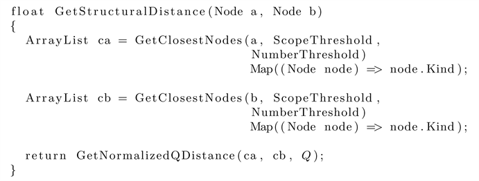
Based upon the above functions, we have defined a deterministic structural similarity algorithm that runs in where n is the number threshold for selecting the closest nodes. In the next section we will explain how we can use structural similarity in the matching procedure.
4.3. Matching Nodes between ASTs
In the previous section we defined how we can separate measuring similarity into two by defining content similarity and structural similarity. These similarities are used in the matching algorithm to determine the certainty of which node is the best match for some other node. This means that for each node n in a tree T we try to find some matching node m in tree T’. At which point we can say that its worst time complexity will be at least . The algorithm we present is based on the matching algorithm in “A 3-way merging algorithm for synchronizing ordered trees - the 3DM merging and differencing tool for XML’’ by Tancred Lindholm [5] . However, it is fundamentally different in the actual matching stage as only its post-processing stage is similar. Therefore, we will explain the matching stage in-depth while briefly explaining the post-processing stage.
4.3.1. Finding the Potential Candidates for a Node
Although the process of finding matches for a node is a part of the matching stage, it is where we will use the content and structural similarity algorithms, therefore it closely relates to the previous chapter and is the reason why we will introduce it first. The match finding algorithm can be divided in two components: finding exact or hash-based matches and finding fuzzy matches.
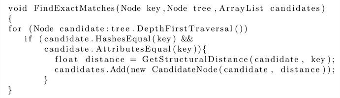
Finding a hash-based is as its name indicates, based on hash values. This is a relatively simple process where for each node n tree T we look for a matching node m tree T’ by comparing their content hash and structural hash for equality. Since we are looking for an exact match, we should compare more than hash values in case of hash collisions. Therefore, we also check for equality for the following node attributes: node kind, total node information weight, total (sub)tree size and total length of text contained within the node. Although unequal nodes can still be a match, it is very unlikely and we will see in the matching stage how we will deal with such collisions. A basic implementation of a function that provides a list of exact or hash based matches can be as follows:
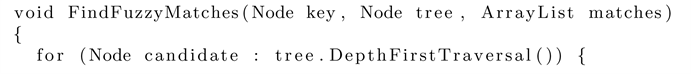
In case no exact or hash-based matches are found, then we should look for fuzzy matches as a node might have changed slightly and one is similar to a certain degree. This degree we define as the fuzzy match threshold and is necessary to make sure that we will not match nodes that are too dissimilar. In our algorithm, we found a fuzzy matching threshold of 0.4 to be adequate as it produced the best matching results without getting false matches.
When we iterate through a tree looking for a match, we first check whether the candidate’s node kind is the same as the node we are trying to match to. If it is not the same, we discard the node since it is an impossible match. Next we use fuzzy matching threshold to compare to a weighted similarity between the possible candidate and the node, using the content and structural similarity algorithms we defined in the previous section. This weighted similarity value calculated by defining a weight for both the content similarity and structural similarity, denoted Wc and Ws. These weights can then be used to define the weight similarity between two nodes n and m, such that:
Using the above similarity function, for a node n we add a candidate m to our set of candidate matches if where is the fuzzy matching threshold. Similar to finding exact matches, we traverse a tree looking for a match and make sure if the match is possible by comparing node kinds. An example of its implementation can be:

From the matches that are either an exact or fuzzy match, we select the best match based upon its similarity distance. However, under the above definitions a node can be part of multiple matches. The entire match procedure is more complicated and can be divided into three sub-procedures and how we will deal with multiple matches will be explained throughout the next few sections.
4.3.2. Matching Nodes with Potential Candidates
Our matching algorithm is partially based on the matching algorithm used in 3DM, and we explain the differences as well as why a different approach was chosen. The fundamental thing we should realize is that if a match is found between two nodes, then the entire subtree probably matches as well. Which is why we should consider matching based on subtrees and is also where the first difference is with 3DM as we do not use a so called truncated subtree as stated by Tancred Lindhol [5] :
Let T be a tree, and T’ a tree for which all nodes : . Let Ts be the tree which is obtained from T’ by replacing all leaf nodes in T’ with the subtrees of T rooted at the leaf nodes. T’ is a truncated subtree of T iff Ts is a subtree of T.
Instead of a truncated subtree, we designed the algorithm around a complete subtree. The procedure works by iteratively traversing T in breadth-first-order and looking for matching nodes (or entire subtrees) in T’. Usually several matching subtree candidates are found, in which case the subtree with the lowest distance is used, unlike 3DM where it selects the subtree with the most nodes. In case there are multiple matches with the same lowest distance, another selection is performed based on previous matches done. For example, if the left siblings of both nodes are matched to each other, then we prefer to use that match over another match with the same distance.
Once the best matching subtree has been selected, the subtree nodes in T and T’ are matched if they are structurally equal. We already have made a definition for this when we defined a structural hash for each node, representing the structure of its subtree. This allows us to check for equality in , and all we have to do after match all the corresponding descendant nodes. In addition, the subtree nodes in T are also tagged with a subtree tag, which uniquely identifies the subtree. This is done to keep track of of the matched subtrees for later the post-processing stages. However, if there is no structural equality between the matched nodes, the procedure iterates again for each child node of the matched node, i.e. the nodes that were not yet matched. We will now look at each step of the matching stage in some detail.
The tree traversal starts with breadth-first traversal using a queue, starting each node , we take the most similar candidate which is found by searching for matches for some node m in T’. Nodes who match exactly (based upon procedure FindExactMatches are considered first. If no such nodes are found, we return all candidate nodes for which , provided by FindFuzzyMatches and are then sorted by their distance similarity. We then attempt to match the entire subtree to the most similar candidate if they are structurally equal based on their structural hash. Should a hash collision occur, we perform a rollback, unset all matches there were set in the subtree (identified by subtree tag) and attempt matching to the next best candidate if it exists. Otherwise, if no match was found or match was made that was no structurally equal, then we enqueue all child nodes of mi and iteratively repeat the process until the queue is empty. The entire procedure is described in pseudocode below:

4.3.3. Removing Matches of Small Copies
In our matching algorithm defined above, multiple nodes mi in tree T’ can be matched with the same node n in tree T. A common case in matching source is that curly brackets get matched together, even though they are structurally barely related or not related at all to each other. Although this is completely fine, we would like to be able to identify which match contains the original nodes and remove copied matches such that they can be inserted in the merging algorithm instead. The first post-processing procedure called RemoveSmallCopies stage deals with this issue by defining a copy threshold on how much data must be duplicated before we can consider it a copy rather than an insertion. The procedure checks all nodes in T’, whose base match in T has several matches in T’ (i.e. the base match is copied). If the copied subtree of T to which the node belongs has an information weight smaller than a certain threshold, the match should be removed and considered inserted instead. The information weight of a node or subtree is the same as we defined in the content similarity section, and is denoted .
Sometimes, the subtrees mi of all matches to a node n are smaller than the copy threshold. In this case we do not want to remove all the matchings, but rather try to identify the original match, and leave it matched. We do it by looking at the neighbors of the match’s subtree root: if the left and right siblings match the left and right siblings in T, we add the information weight of the matching trees to that of the candidate for match removal. Candidates that gets an information weight higher than the copy threshold, or the candidate with the highest information weight in case all subtrees have an information weight lower than the copy threshold, will be considered valid matches.
4.3.4. Matching Similar Unmatched Nodes
Based on the matchings that were made before in the matching stage, we can attempt to make additional matchings by looking at neighboring matches. The second post-processing procedure called MatchSimilarUnmatched does exactly that, and its task is to find such pairs of nodes and match them accordingly. The procedure is relatively simple was defined as follows [5] :
Let m and n be a pair of unmatched nodes. If the parents of m and n are matched, and if either the left or right siblings (if they exist) of m and n are matched, m and n should be matched. If neither siblings match (possibly because they do not exist), we will also match the nodes if both m and n are the last or first node in the child list. Finally, if the child nodes of both m and n match each other, then m and n should be matched as well.
4.3.5. Time Complexity Analysis of the Full Algorithm
We conclude the presentation of the matching algorithm by analyzing its complexity. For the sake of the analysis we divide the matching algorithm in four steps: structural similarity, content similarity, matching subtrees, and removing small copies and matching similar unmatched nodes. In reality the similarity algorithms are included in the matching subtrees step. Without further a due, based upon the descriptions of the algorithms described in previous sections, we can define their time complexity as:
1) The procedure GetStructuralSimilarity is performed in , where a circumference threshold. This is trivially defined, since we visit at most nodes and then sort them in .
2) The procedure GetContentSimilarity is performed in , where S is the length of the string content with a subtree, a the branching factor of the trees and the subtree has levels, such that the total number of leaves is . This is true since similarity is measured per token pair which can only be done from the leaves. The top node has work associated with it, the next level has work associated with each of a nodes and so forth.
3) The procedure MatchSubTrees is performed in . For each node n in a tree T we look for a matching node m in tree T’, where we have to check for both structural similarity and content similarity in the worse case. Therefore, it’s time complexity is using previous definitions.
4) The procedures RemoveSmallCopies and MatchSimilarUnmatched are performed in and respectively as has been proven before [5] .
Our full algorithm consists of the above procedures, and in a reasonable matching case we can make the assumption that; is so small compared to the tree size that the time complexity of GetStructuralSimilarity can be reduced to . Therefore, we can write the worst case time complexity of the full algorithm as follows:
However, this is absolute worst case where no matching subtrees are found at all, which is never the case any realistic matching scenario. Typically we will be able to to match entire subtrees at once in time in the procedure MatchSubTrees, and if we assume there are D matched subtrees, we can define the full algorithms worst time complexity as , where is the amount of syntax tokens.
4.4. Merging Matched ASTs
Merging ASTs is the last stage of the algorithm and is where merging is performed based on the matches that were made in the matching stage. During this stage, certain ambiguities may occur which is referred to as a conflict. A typical case of a conflict is that a merging algorithm cannot make sense of the ASTs due to dissimilar structure, and in our case it can happen when no matches were found for a certain node that already existed. This is the reason why the matching stage of the algorithm is can be considered the most important. Nonetheless, the merging stage is also important due to considerations such as minimal distance and time complexity.
In the Section 4.3 we introduced several algorithms how similarity can be measured between nodes such that it can be used to match nodes between two given trees. Based upon these matches, perform a merging algorithm that merges these two trees into a merged one. Due to the amount of research already performed on merging tree structures, there is actually no need for us to design our own algorithm. Which is why we have chosen an existing merging algorithm that is compatible with our matching algorithm; “A 3-way merging algorithm for synchronizing ordered trees” by Tancred Lindholm [5] .
The general idea of the algorithm he proposes is to traverse the trees T and T’ simultaneously such that matched nodes are traversed at the same time. Each iteration of the traversal outputs a merge of two matched nodes that are currently being visited to TM. In addition, the concept of a tree cursor is introduced which points to the current position in a tree. The tree cursor may point to a null node, which means the cursor is inactive. Cursors are denoted by CT, where T is the tree that will be traversed by the cursor, while the the null node is denoted ε. For example, suppose we have two trees T and T’, then the cursors are written as and .
Nodes that are put together for merging are called a merge pair and denoted , where n and m are the nodes in the pair. Merge pairs can also contain one null node, which represents an existing node for which we could not find a match. In this case, the merge pair is denoted . Lastly, the merge algorithm assumes that the trees T and T’ are non-empty, that the matchings M and M’ exist, and all cursors are initially positioned at the root of their associated tree. These are the initial conditions for the algorithm and our matching algorithm defined in the previous section provides such conditions and is therefore compatible with the merging algorithm.
5. Testing and Evaluation
Now that the problem has been stated and its theoretical solution has been proposed, the real-world experiments and their results can be presented which have been carried out as a demonstration that the solution truly does work. In this chapter, we will explain how we have implemented the solution and what environment is required to be able to use the theoretical solution.
As an example programming language for the research, Microsoft’s. NET language C# has been chosen as it is a well defined language and is commonly used in real-world applications. Our theoretical solution defined in Chapter 4 assumes that a given AST as its input, which means a source code parser is required. Although it is possible to write our own parser, we have decided not to reinvent the wheel. Instead, we have chosen Roslyn as our parser, which was recently released (July 2015). Since its release Roslyn is the official C# language parser and compiler, developed by Microsoft over the past few years. In addition, we have chosen MurmurHash3 as our hashing algorithm due to its simple implementation, fast performance and low collision rate. Lastly, it should be mentioned that no other libraries were used such that the implementation can be replicated in any other programming language provided that a parser is available.
5.1. Overview of the Implementation
For testing and evaluation, the algorithm was implemented in C# and runs on both. NET and Mono. C# was selected due mainly to the availability of a parser that could parse C#, namely Roslyn. Although it would have been possible to use another programming language as well, C# is similar to Java and both are widely accepted in the current generation. In addition, thanks to several. NET standard library features such as LINQ it saved a lot of time implementing basic algorithms such as sorting algorithms. In this section, we give a brief overview of the structure of the implementation. Readers who are interested in the details of the implementation are recommended to start by reading this section to get an overview and thereafter to read trough the source code.
The main class in the framework is Matching.cs, where you will find implementations of the matching algorithms can be found, such as MatchSubTrees, RemoveSmallCopies and MatchSimilarUnmatched which were presented in the previous chapter. The Matching class constructor takes two parameters, a base node and a branch node where each of them represents the root of a source code file.
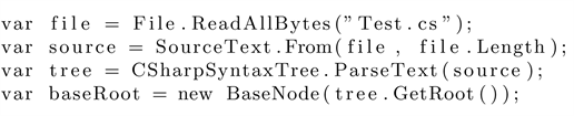
Roots of both a base node and branch node can be constructed in a simple manner by calling its constructor and passing a syntax tree that was parsed by Roslyn. An example of constructing such a root node would be:
Most of the implementation of how nodes are built from their constructor can be found in Node.cs, while the derivations BaseNode and BranchNode have additional minor functionality and their definitions can be found in BaseNode.cs and BranchNode.cs.
The high-level similarity algorithms can be found in Similarity.cs, such as GetContentDistance, GetStructuralDistance and GetClosestNodes. The high-level algorithms can make use of certain low-level similarity algorithms that can be found in Distance.cs. The low-level algorithms implemented are Q-gram, Levenshtein edit distance, Jaro-Wrinkler edit distance, Sift4 edit distance, and Zhang and Shasha’s tree edit distance algorithms [11]. These algorithms have been implemented to thoroughly test real-world examples in terms of matching accuracy, consistency and time complexity. One of these real-world examples will be shown in the next section.
5.2. A Real-World Example of Matching Two Files
Although we have tested many real-world cases throughout our research, we will show one rather extreme example where many changes were applied to a file in order to demonstrate how robust the matching algorithm is. As the edited file is a lot bigger than the original, we will simply the source code and only show the areas where the code actually changed. In short, a new using directive was added, the class identifiers were swapped, the order of methods was changed significantly and other minor changes within those methods. This includes changes a method declaration identifier and return type, while writing an additional invocation expression with two parameters:
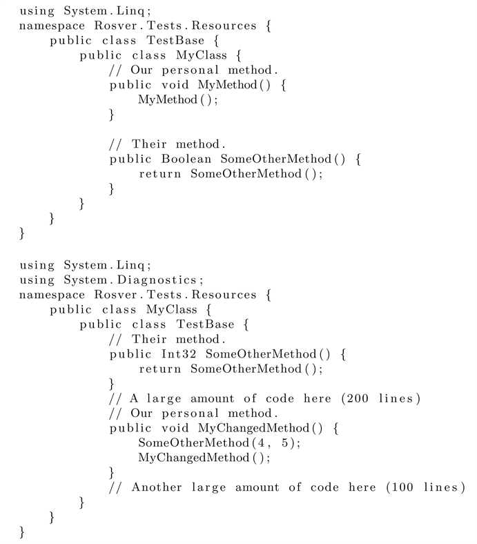
In the above example, we have a matching rate of 100%. Which means that we were able to matched every node that existed in the original source code file, in this case 76 out of all 76 nodes. The accuracy of our matching algorithm in this example (and many others) is quite high considering how much the environment changed.
6. Conclusion and Future Work
Throughout this article, we have introduced several existing version control systems and explained why they need improvement in certain areas. One of those areas is matching source code while truly understanding its actual content which is the main topic we have chosen for this article. As such, we have defined a problem statement as to what problems need to be solved and which requirements the solution must conform to. Although there are already several existing matching and merging algorithms, none of these target programming languages as a special case such that they can be reasoned about in a more specific way.
The solution we present consists of a similarity algorithm and matching algorithm that are partially based on the 3DM merging and differencing tool for XML [5] . Although several concepts were derived from it, our solution is fundamentally different in both implementation and accuracy for the similarity and matching algorithm. We make use of both a content and structural hash, based on the concept of a Merkle tree [8] , such that equality checks can be performed in constant time, where entire subtrees can be matched at once as long as hash collisions are avoided. In addition, we define structural similarity of a node based on its circumference within a certain scope and size threshold, and perform a linear time similarity algorithm on its circumference that surprisingly accurately approximates the distance. Content similarity has also been defined and is measured by measuring similarity of each token’s content rather than an entire string or line of text at once.
The matching algorithm accurately finds matches between two trees through hash-based matching and fuzzy matching that uses the similarity algorithms. Something that also should be noted is that all algorithms designed in this article have been defined as iterative procedures rather than recursive procedures in order to avoid stack overflows for large source code files. Examples of this are use of breadth-first-search based on a queue and depth-first-search based on a stack.
The theoretical solution has been thoroughly tested by developing a framework based on the theory defined in Chapter 4. Using this framework, tests on several real-world examples have been performed, of which one of them has been presented in Chapter 5. The outcome of article experiments were satisfying results, where source code files were often matched optimal and others near-optimal. In some cases, matches were not found due to the text of tokens being too dissimilar. Based on these results, a more advanced algorithm could be designed that uses the values of content similarity and structural similarity in a different manner.
We have addressed all problems and requirements stated in the problem description by having defined several new algorithms that handle source code matching efficiently and accurately. However, there is still a lot of points for improvement in them, such improving the content similarity algorithm. The amount of trivia surrounding a syntax token can be a huge amount compared to the actual token, the content similarity algorithm does not consider this. In the case of a large difference in the trivia, certain tokens may not be matched due to trivia being too dissimilar. A possible solution would be to consider trivia separately and giving them a small weight compared to the syntax token itself.
Furthermore, it should be investigated whether structural similarity can be performed in linear time rather than line arithmic time. The AST should already have been sorted in depth-first-order by the parser, such that any particular subtree can perhaps be generated in linear time as well by possibly using a linked list structure.
In conclusion, we have designed a matching algorithm that performs reasonably to very well in a real-world environment in terms of both time complexity and matching precision. This article was inspired by Wouter Swierstra who wrote the article “The Semantics of Version Control” [3] and the solution algorithm has been based on the thesis of Tancred Lindholm, who defined a three-way merging algorithm [5] . The author intends to develop algorithms defined in this thesis further and strive to find a solution that will truly be an improvement for existing version control systems, such that developers can work more efficiently in software projects.
Cite this paper
van den Berg, J. and Haga, H. (2018) Matching Source Code Using Abstract Syntax Trees in Version Control Systems. Journal of Software Engineering and Applications, 11, 318-340. https://doi.org/10.4236/jsea.2018.116020
References
- 1. O’Sullivan, B. (2009) Making Sense of Revision-Control Systems. Communications of the ACM, 52, 56-62. https://doi.org/10.1145/1562164.1562183
- 2. Loh, A. and Swierstra, W. (2008) A Principled Approach to Version Control. http://www.andres-loeh.de/fase2007.pdf
- 3. Jiang, L., Misherghi, G., Su, Z. and Glondu, S. (2007) DECKARD: Scalable and Accurate Tree-Based Detection of Code Clones. Proceedings of 29th International Conference on Software Engineering, Minneapolis, 20-26 May 2007, 96-105.
- 4. Reynolds, J., et al. (2002) Separation Logic: A Logic for Shared Mutable Data Structures. Proceedings of the 17th Annual IEEE Symposium on Logic in Computer Science, Copenhagen, 22-25 July 2002, 55-74. https://doi.org/10.1109/LICS.2002.1029817
- 5. Lindholm, T., et al. (2001) A 3-Way Merging Algorithm for Synchronizing Ordered Trees—The 3 dm Merging and Differencing Tool for X ml. Master’s Thesis, Helsinki University of Technology, Otaniemi.
- 6. Zhang, K. and Shasha, D. (1997) Approximate Tree Pattern Matching. Pattern Matching in String, Trees and Arrays, Oxford University Press, Oxford, 341-371.
- 7. Rochkind, M. (1975) The Source Code Control System (SCCS). Software Engineering, 1, 364-370. https://doi.org/10.1109/TSE.1975.6312866
- 8. Merkle, R. (1979) Secrecy, Authentication, and Public Key Systems. Stanford University, Stanford, 86-95.
- 9. Zhang, K. and Shasha, D. (1989) Simple Fast Algorithms for the Editing Distance between Trees and Related Problems. SIAM Journal on Computing, 18, 1245-1262. https://doi.org/10.1137/0218082
- 10. Demaine, E.D., Mozes, S., Rossman, B. and Weimann, O. (2009) An Optimal Decomposition Algoritm for Tree Edit Distance. ACM Transactions on Algorithms, 6, 2:1-2:19.
- 11. Fast Algorithms for the Unit Cost Editing Distance between Trees (1990) Comparison and Evaluation of Clone Detection Tools. Journal of Algorithms, 4, 581-621.