Journal of Software Engineering and Applications
Vol.09 No.05(2016), Article ID:66661,17 pages
10.4236/jsea.2016.95015
A Generic Graph Model for WCET Analysis of Multi-Core Concurrent Applications
Robert Mittermayr, Johann Blieberger
Institute of Computer Aided Automation, TU Vienna, Vienna, Austria

Copyright © 2016 by authors and Scientific Research Publishing Inc.
This work is licensed under the Creative Commons Attribution-NonCommercial International License (CC BY-NC).
http://creativecommons.org/licenses/by-nc/4.0/


Received 29 March 2016; accepted 20 May 2016; published 23 May 2016
ABSTRACT
Worst-case execution time (WCET) analysis of multi-threaded software is still a challenge. This comes mainly from the fact that synchronization has to be taken into account. In this paper, we focus on this issue and on automatically calculating and incorporating stalling times (e.g. caused by lock contention) in a generic graph model. The idea that thread interleavings can be studied with a matrix calculus is novel in this research area. Our sparse matrix representations of the program are manipulated using an extended Kronecker algebra. The resulting graph represents multi-threaded programs similar as CFGs do for sequential programs. With this graph model, we are able to calculate the WCET of multi-threaded concurrent programs including stalling times which are due to synchronization. We employ a generating function-based approach for setting up data flow equations which are solved by well-known elimination-based dataflow analysis methods or an off-the-shelf equation solver. The WCET of multi-threaded programs can finally be calculated with a non-linear function solver.
Keywords:
Worst-Case Execution Time Analysis, Program Analysis; Concurrency, Multi-Threaded Programs, Kronecker Algebra

1. Introduction
It is widely agreed that the problem of determining upper bounds on execution times for sequential programs has been more or less solved [1] . With the advent of multi-core processors scientific and industrial interest focuses on analysis and verification of multi-threaded applications. The scientific challenge comes from the fact that synchronization has to be taken into account. In this paper, we focus on how to incorporate stalling times in a WCET analysis of shared memory concurrent programs running on a multi-core architecture. The stress is on a formal definition and description of both, our graph model and the dataflow equations for timing analysis.
We allow communication between threads in multiple ways e.g. via shared memory accesses protected by critical sections. Anyway, we use a rather abstract view on synchronization primitives. Modeling thread interactions on the hardware-level is out of the scope of this paper. A lot of research projects have been launched to make time predictable multi-core hardware architectures available. Our approach may benefit from this research.
Previous work done in the field of timing analysis for multi-core (e.g. [2] ) assumes that the threads are more or less executed in parallel and the threads do not heavily synchronize with each other, except when forking and joining. Our approach supports critical sections and the corresponding stalling times (e.g. caused by lock contention) in the heart of its matrix operations. Forking and joining of threads can also easily be modeled. Thus, our model is suitable for systems from a concurrent to a (fork and join) parallel execution model. Anyway, the focus in this paper is on a concurrent execution model.
The idea that thread interleavings and synchronization between threads can be studied with a matrix calculus is novel in this research area. Our sparse matrix representations of the program are manipulated using a lazy implementation of our extended Kronecker algebra. In [3] the Kronecker product is used in order to model synchronization. Similar to [4] [5] , we describe synchronization by our selective Kronecker products and thread interleavings by Kronecker sums. The first goal is the generation of a data structure called concurrent program graph (CPG) which describes all possible interleavings and incorporates synchronization while preserving completeness. In general, our model can be represented by sparse adjacency matrices. The number of entries in the matrices is linear in their number of lines. In the worst case, the number of lines increases exponentially in the number of threads. The CPG, however, contains many nodes and edges unreachable from the entry node. If the program contains a lot of synchronization, only a very small part of the CPG is reachable. Our lazy implementation computes only this part which we call reachable CPG (RCPG). The implementation is very memory-efficient and has been parallelized to exploit modern many-core hardware architectures. These optimizations speed up processing significantly.
RCPGs represent concurrent and parallel programs similar as control flow graphs (CFGs) do for sequential programs. In this paper, we use RCPGs to calculate the WCET of the underlying concurrent system. In contrast to [4] , we (1) adopt the generating functions based approach of [6] for timing analysis and (2) are able to handle loops. For timing analysis, we set up a data flow equation for each RCPG node. It turns out that at certain synchronizing nodes, stalling times (e.g. caused by lock contention) can be formulated within dataflow equations as simple maximum operations. Choosing this approach, the calculated WCET includes stalling time. This is in contrast to most of the work done in this field (e.g. [2] ), which usually adopts a partial approach, where stalling times are calculated in a second step. We successively apply the following steps:
1. Generate CFGs out of binary or program code (cf. Subsection 2.1).
2. Generate RCPG out of the CFGs (cf. Section 3).
3. Apply hardware-level analysis based on the RCPG. Such an analysis may take into account e.g. shared resources like memory, data caches, and buses, and other hardware components like instruction caches and pipelining. Annotate this information at the corresponding RCPG edges. As mentioned above, this step is out of scope of this paper. Anyway, in order to get tight bounds this step is necessary (cf. [7] ). Some of these analyses (e.g. cache analysis) may be performed together with the next step.
4. Establish and solve dataflow equations based on the RCPG (cf. Section 4). Stalling times are incorporated via the equations.
Similar to [6] and [8] , which provide exact WCET for sequential programs, our approach calculates an exact worst-case execution time for concurrent programs running on a multi-core CPU (not only an upper bound) provided that the number of how often each loop is executed, the execution frequencies and execution times of the basic blocks (also of the semaphore operations p and v)1 on RCFG level are known, and hardware impact is given. We assume timing predictability on the hardware level as discussed e.g. in [8] .
The outline of our paper is as follows. In Section 2, refined CFGs and Kronecker algebra are introduced. Our model of concurrency, some properties, and our lazy approach are presented in Section 3. Section 4 is devoted to WCET analysis of multi-threaded programs. An example is presented in Section 5. In Section 6, we survey related work. Finally, we draw our conclusion in Section 7.
2. Preliminaries
In this paper, we refer to both, a processor and a core, as a processor. Our computational model can be described as follows. We model concurrent programs by threads which use semaphores for synchronization. We assume that on each processor exactly one thread is running and each thread immediately executes its next statement, if the thread is not stalled. Stalling may occur only in succession of semaphore calls.
Threads and semaphores are represented by slightly adapted CFGs. Each CFG is represented by an adjacency matrix. We assume that the edges of CFGs are labeled by elements of a semiring. A prominent example for such semirings are regular expressions [9] describing the behavior of finite state automata.
The set of labels  is defined by
 , where
  is the set of ordinary (non-synchronization) labels and
  is the set of labels representing semaphore calls (
 and
and  are disjoint). In order to model
e.g. a critical section usually two or more distinct thread CFGs refer to the same semaphore [10] . The operations on the basic blocks are , and * from a semiring [9] . Intuitively, these operations model consecutive program parts, conditionals, and loops, respectively.
2.1. Refined Control Flow Graphs
CFG nodes usually represent basic blocks [11] . Because our matrix calculus manipulates the edges, we need to have basic blocks on the (incoming) edges. A basic block consists of multiple consecutive statements without jumps. For our purpose, we need a finer granularity which we achieve by splitting edges. We apply it to basic blocks containing semaphore calls (e.g.  and
and ) and require that a semaphore call
  has to be the only statement on the corresponding edge. Roughly speaking, edge splitting maps a CFG edge e whose corresponding basic block contains k semaphore calls to a subgraph
  , such that each
  represents a single semaphore call, and
  and
and  represent the consecutive parts before and after
 , respectively (
 ). Applying edge splitting to a CFG results in a refined control flow graph (RCFG). Note that a shared memory access aware analysis requires additional edge splitting for e.g. shared variables as done in [12] .
In the following, we use the labels as defined above as representatives for the basic blocks of RCFGs. To keep things simple, we refer to edges, their labels, the corresponding basic blocks and the corresponding entries of the adjacency matrices synonymously. In a similar fashion, we refer to nodes, their row and column numbers in the corresponding adjacency matrix synonymously. A matrix entry a in row i and column j is interpreted as a directed edge from node i to node j labeled by a.
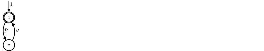
In Figure 1(a) a binary semaphore is depicted. In a similar way it is possible to model counting semaphores allowing n non-blocking p-calls. Entry nodes have an incoming edge with no source node. A double circled node indicates that it is a final node. In the remainder, we use the RCFGs of the threads A and B presented in the Figure 1(b) and Figure 1(c), respectively, as a running example.
2.2. Modeling Synchronization and Interleavings
Kronecker product and Kronecker sum form Kronecker algebra. In the following, we define both operations. Proofs, additional properties, and examples can be found in [13] [14] . From now on, we use matrices out of  only.
only.
 (a) (b) (c)
Figure 1. RCFGs of a binary semaphore and the threads A and B. (a) Binary semaphore; (b) RCFG of thread A; (c) RCFG of thread B.
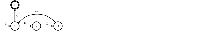
Definition 1 (Kronecker Product) Given a m-by-n matrix A and a p-by-q matrix B, their Kronecker product  is a mp-by-nq block matrix defined by
Kronecker product allows to model synchronization [3] . Properties concerning connectedness when applied to directed graphs can be found in [15] .
Definition 2 (Kronecker Sum) Given a matrix A of order2 m and a matrix B of order n, their Kronecker sum  is a matrix of order mn defined by
 , where
  and
and  denote identity matrices of order m and n, respectively.
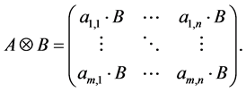
The Kronecker sum calculates all possible interleavings of two concurrently executing automata (see [16] for a proof) even for general CFGs including conditionals and loops. In Figure 2 the Kronecker sum of the threads A and B depicted in Figure 1 is shown. It can be seen that the Kronecker sum calculates all possible interleavings of the two threads. In particular, note that thread A’s loop is copied five times (B’s number of nodes). We write  to refer to the i-th copy of label l. If it is not clear in the context to which thread a label l belongs, we write
  to denote that l belongs to thread X. In particular, this is necessary for semaphore operations which are usually called by at least two threads. Otherwise the executing thread would be unknown.
3. Concurrent Program Graphs
Our system model consists of a finite number of threads and semaphores which are both represented by RCFGs. Threads call semaphores in order to implement synchronization or locks i.e. mutual exclusion for access to shared resources like shared variables or shared buses. The RCFGs are stored in form of adjacency matrices. The matrices have entries which are referred to as labels  as defined in Section 2.
Formally, the system model consists of the tuple , where
  is the set of RCFG adjacency matrices describing threads,
  refers to the set of RCFG adjacency matrices describing semaphores, and
denotes the set of labels out of the semiring defined in the previous section. The labels (or matrix entries) of the
i-th thread's adjacency matrix  are elements of
 , whereas the labels (or matrix entries) of the j-th
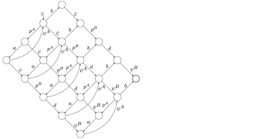
Figure 2. Kronecker sum  of threads A and B.
synchronization primitive's adjacency matrix  are elements of
 . The matrices are manipulated by
using conventional Kronecker algebra operations together with extensions which we define in the course of this section.
A concurrent program graph (CPG) is a graph 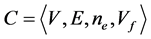 with a set of nodes V, a set of directed edges
 , a so-called entry node
  and a set of final nodes
 . The sets V and E are constructed out of the elements of
 . Details on how we generate the sets V and E follow below. Similar to RCFGs the edges of CPGs are labeled by
 .
.
In general, a thread’s CPG may have several final nodes. We refer to a node without outgoing edges as a sink node. A sink node appears as zero line in the corresponding adjacency matrix. A CPG’s final node may also be a sink node (if the program terminates). However, sink nodes and final nodes can be distinguished as follows. We
use a vector determining the final nodes of thread i, namely . In addition, vector
  determines the final
node of synchronization primitive j. Both have ones at places q, when node q is a final node, zeros elsewhere.
Then the vector  determines the final nodes of the CPG.
In the remainder of this paper, we assume that all threads do have only one single final node. Our results, however, can be generalized easily to an arbitrary number of final nodes.
3.1. Generating a Concurrent Program’s Matrix
Let  and
and  refer to the matrices representing thread i and synchronization primitive (e.g. semaphore) i, respectively. According to Figure 1(a) we have for binary semaphore i the adjacency matrix
 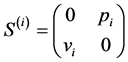 of order two. We obtain the matrix T representing k interleaved threads and the matrix S repre- senting r interleaved synchronization primitives by
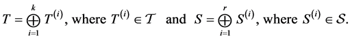
Because the operations  and
and  are associative [4] , the corresponding n-fold versions are well defined. Hence, we can apply the operations on multiple matrices (representing threads and synchronization primitives).
In the following, we define the selective Kronecker product which we denote by . This operator synchronizes only labels identical in the two input matrices.
Definition 3 (Selective Kronecker Product) Given an m-by-n matrix A and a p-by-q matrix B, we call  their selective Kronecker product. For all
  let
let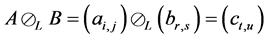 , where

The ordinary Kronecker product on the automata-level calculates the product automaton. In contrast, the selective Kronecker product is defined for only one active component. One thread executes the synchronization primitives’ operations. The synchronization primitive itself is a passive component. In contrast to the ordinary Kronecker product, the selective Kronecker product is defined such that a label l in the left operand is paired
with the same label in the right operand and not with any other label in the right operand and for 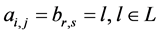
the resulting entry is l and not . Definition 3 is defined for a set of labels L. In the following, we use it exclusively for
 . Thus, we use this operation only for labels referring to synchronization primitive calls. Used that way, the selective Kronecker product ensures that, e.g., a p-call to semaphore i, i.e. a
  -call, in the left operand is paired with the corresponding
  -operation in the right operand and not with any other label (e.g.
  of a semaphore
 ) in the right operand.
Definition 4 (Filtered Matrix) We call  a filtered matrix and define it as a matrix of order
  containing entries of
  of
of  and zeros elsewhere:

The adjacency matrix representing a program is referred to as P. As stated in [4] [17] , P can be computed efficiently by
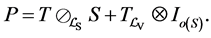
Intuitively, the selective Kronecker product term on the left allows for synchronization between the threads represented by T and the synchronization primitives S. Both T and S are Kronecker sums of the involved threads and synchronization primitives, respectively, in order to represent all possible interleavings of the concurrently executing threads. The right term allows the threads to perform steps that are not involved in synchronization. Summarizing, the threads (represented by T) may perform their steps concurrently, where all interleavings are allowed, except when they call synchronization primitives. In the latter case the synchronization primitives (represented by S) together with Kronecker product ensure that these calls are executed in the order prescribed by the finite automata (FA) of the synchronization primitives. So, for example, a thread cannot do semaphore calls in the order v followed by p when the semaphore FA only allows a p-call before a v-call. The CPG of such an erroneous program will contain a node from which the final node of the CPG cannot be reached. This node is the one preceding the v-call. Such nodes can easily be found by traversing CPGs. Thus, deadlocks of concurrent systems can be detected with little effort [12] [17] .
Until now the following synchronization primitives have been successfully applied. In [4] [12] semaphores are the only synchronization primitives. In [17] the approach is extended in order to model Ada’s protected objects, too. Finally, in [5] it is shown that barriers can be used as synchronization primitives. In the latter paper it is also presented that initially locked and unlocked semaphores can be incorporated to our Kronecker algebra-based approach.
It can easily be shown that CPGs have at most  nodes and at most
  edges, if k is the number of threads and each thread has n nodes in its RCFG. Hence, each CPG has a sparse adjacency matrix
 .
.
Thus, memory saving data structures and efficient algorithms suggest themselves. In the worst-case, however, the number of CPG nodes increases exponentially in k.
3.2. Lazy Implementation of Kronecker Algebra
In general, a CPG contains unreachable parts if a concurrent program contains synchronization. This can be summarized as follows: The way we adopt the Kronecker product limits the number of possible paths such that the p- and v-operations are present in correct p-v-pairs in the RCPG. In contrast 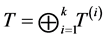 contains all
possible paths even those containing semantically wrong uses of the synchronization primitive (e.g. semaphore) operations. This contrast can be seen in our running example in Figure 2 and Figure 3. The Kronecker sum of thread A and B in Figure 2 contains five copies of thread A’s loop, whereas the RCPG in Figure 3 contains this loop only three times. It can be easily seen that the latter reflects the correct use of the semaphore operations.
Choosing a lazy implementation for the matrix operations ensures that, when extracting the reachable parts of the underlying graph, the overall effort is reduced to exactly these parts. By starting from the RCPG’s entry node and calculating all reachable successor nodes, our lazy implementation exactly does this [4] . Thus, for example, if the resulting RCPG’s size is linear in terms of the involved threads, only linear effort will be necessary to generate the RCPG.
4. WCET Analysis on RCPGs
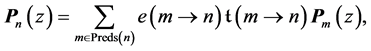
In order to calculate the WCET of a concurrent program, we adopt the generating functions based approach introduced in [6] . We generalize this approach such that we are able to analyze multi-threaded programs. Each node of the RCPG is assigned a dataflow variable and a dataflow equation is set up based on the predecessors of the RCPG node. A dataflow variable is represented by a vector. Each component of the vector reflects a processor and is used to calculate the WCET of the corresponding thread. Recall that only one single thread is allocated to a processor. Even though RCPGs support multiple concurrent threads on one CPU also, we restrict
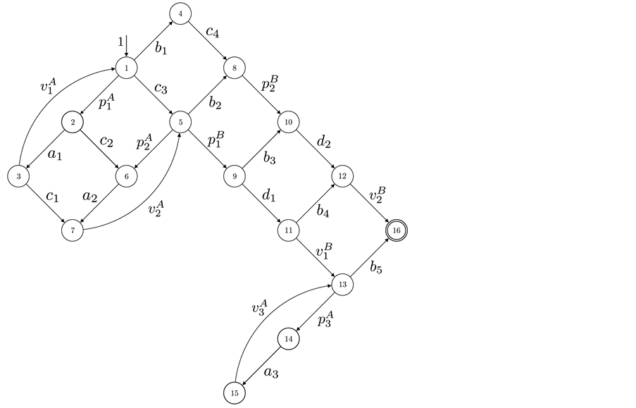
Figure 3. RCPG.
the WCET analysis to one thread per processor. This assumption eases the definition of the dataflow equations and it is not a restriction from our approach itself.
4.1. Execution Frequencies
In the remaining part of the paper, we will use execution frequencies [6] . The execution frequency  is a measure of how often the edge
  is taken compared to the other outgoing edges of node k. Thus, each execution frequency is a rational number. Its values range from 0 (which models a dead path) to 1, i.e.,
 . For each node k, it is required that the execution frequencies of all outgoing edges sum to 1. If node k has at least two outgoing edges, then we have a so-called node constraint
 . We assign a variable to each
 . A concrete value is assigned to each of these variables during the maximization process which is described below in Section 4.6. If a node m has only one outgoing edge to node n, then the execution frequency
  is statically known and neither a node constraint nor an additional variable for the execution frequency is needed.
4.2. Loops
Let  refer to the set of natural numbers including zero, i.e.,
 . From now on, we use the variable
  to refer to the number of loop iterations of loop i at CFG level. For each loop, we require that
this number is constant3 and statically known. As we have seen in Figure 2, RCPGs contain several copies of basic blocks (in our case edges) and loops in different places.
Since RCPGs model all interleavings of the involved threads, a certain execution of the underlying concurrent program (a certain path in the RCPG) may divide the code of a loop in the CFG among all its copies in the RCPG. In particular, we do not know a priori how a loop will be split among its copies in the RCPG for the path producing the WCET. For this reason, we assign variables (with unknown values) to the number of loop iterations of the loop copies in the RCPG. Later on (during the maximization process), concrete values for this loop iteration variables are chosen such that the execution time is maximized. Note that assigning variables to loop iteration numbers implies that some execution frequencies have also to be considered variable. These execution frequencies also get concrete values during the maximization process.
We refer to the number of loop iterations of the j-th copy of loop i as . This variable denotes the number of how often the loop entry edge of the j-th copy of loop i is executed. The loop entry of the j-th copy (out of n) of loop i gets assigned the execution frequency variable
 , where
 . Note that the variables
  get numerical values during the maximization process. Thus, the execution frequency of each loop entry edge is calculated automatically.
If node m has multiple outgoing loop entry edges for the loops  and there exists exactly one outgoing non loop entry edge, then the execution frequency for the loop entry edge of loop i is
 .
.
Loop Iteration Constraints. Assume CFG loop i is executed  times and n copies (as mentioned above due to the Kronecker sum) of that loop are in the RCPG, then we have the constraint
 . We assume that
the value of variable , i.e., the number of loop iterations on thread (CFG) level is known a priori. The variables
  are used as variables during the maximization process. During the generation of the RCPG it is possible to remember each copy of a CFG loop entry edge. In order to establish the loop iteration constraints, we go through this information.
Loop Exit Constraints. For loop i’s j-th copy we have  iterations. Then we have the loop exit constraint
 , where
  is the sum of execution frequencies of all loop exiting edges of the j-th copy of loop i.
In general, such loop exiting edges do also include edges from other threads which do not execute any part of loop i. Note that we can calculate the loop exit constraints automatically. Our approach does support nested loops [18] which result in non-linear constraints. This is one reason which prohibits applying an ILP-based approach like [8] for solving the concurrent WCET problem.
4.3. Synchronizing Nodes
A thread calling a semaphore’s p-operation potentially blocks [10] . On the other hand, a thread calling a semaphore’s v-operation may unblock a waiting thread [10] . In RCPGs, blocking occurs at what we call synchronizing nodes. We distinguish two types of synchronizing nodes, namely vp- and pp-synchronizing nodes.
Each vp-synchronizing node has an incoming edge labeled by a semaphore v-operation, an outgoing edge labeled by a p-operation of the same semaphore, and these two edges are part of different threads. In this case, the thread calling the p-operation (potentially) has to wait until the other thread’s v-operation is finished.
Definition 5. A vp-synchronizing node is a RCPG node s such that
• there exists an edge  with label
  and
and
• there exists an edge  with label
 ,
,
where k denotes the same semaphore and the edges  and
and  are mapped to different processors, i.e.,
 .
.
For vp-synchronizing nodes, we establish specific data flow equations as described in the following subsection.
Definition 6. A pp-synchronizing node is a RCPG node s such that
• there exists an edge  with label
  and
and
• there exists an edge  with label
 ,
,
where k denotes the same semaphore and the edges  and
and  are mapped to different processors, i.e.,
 .
.
For pp-synchronizing nodes, we establish fairness constraints ensuring a deterministic choice when e.g. the time of both involved CPUs at node s is exactly the same.
4.4. Setting Up and Solving Dataflow Equations
In this section, we extend the generating function based approach of Section 4 of [6] such that we are able to calculate the WCET of concurrent programs modeled by RCPGs. Each RCPG node’s dataflow equation is set up according to its predecessors and the incoming edges (including execution frequency, execution time and in case of vp-synchronizing nodes stalling time).
Let the vector . We write
  to denote the i-th component
  of vector
 . In addition,
  refers to the vector of node x.
Let a be a scalar and let  and
and  be two n-dimensional vectors. The addition and multiplication of vectors and the multiplication of a scalar with a vector are defined as follows:

Definition 7 (Setting up Dataflow Equations) Let  refer to the time assigned to edge
 . In addition, the set of predecessor nodes of node n is referred to as
 .
.
If n is a non-vp-synchronizing node and edge  is mapped to processor k, then
where the kth component of vector  is
is  and the other components are equal to 1.
Let s be a vp-synchronizing node. In addition, let  and
and  be the processors which the edges
  and
and  are mapped to, i.e.,
  and
and .4 Then for

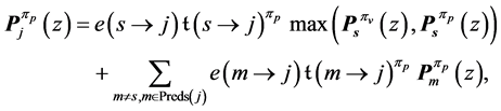
where the first term considers the incoming p-edge and the second term takes into account all other incoming edges of the blocking thread running on processor .
.
The max-operator in Def. 7 is not an ordinary maximum operation for numbers. During the maximization process, we actually do the whole calculation twice. One time, we replace  by
by  and then, we do this calculation using the second solution
 . In the end, the solution with the highest WCET value will be taken.
The entry node’s equation  follows the rules above and, in addition, for n threads adds an
n-dimensional vector .
.
The dataflow equations can intuitively be explained as follows. We cumulate the execution times in an interleavings semantics fashion. One can think of taking one edge after the other. Nevertheless, edges may be executed in parallel and the execution and stalling times are added to the corresponding vector components. In the overall process, we get the WCET of the concurrent program.
The system of dataflow equations can be solved efficiently by applying an algorithm presented in [15] . As a result, we get explicit formulas for the final node. In order to double-check that we calculate a correct solution, we used MathematicaÓ to solve the node equations, too. Both of the two approaches for solving the node equations calculate the same and correct results.
4.5. Partial Loop Unrolling
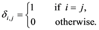
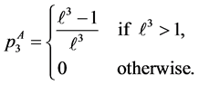
For vp-synchronizing nodes having at least one outgoing loop entry edge5, we have to partly unroll the corresponding loop such that one iteration is statically present in the RCPG’s equations. Partial loop unrolling ensures that synchronization is modelled correctly. Only the unrolled part contains a synchronizing node. Some execution frequencies and equations have to be added or adapted. Edges have to be added to ensure that the original and the unrolled loop behave semantically equivalent. For example, if the original loop was able to iterate  times, then the new construct must also allow the same number of iterations. In order to define some execution frequencies correctly, we are using the Kronecker delta function. We do such partial loop unrolling for our example in the appendix in Subsection 5.2. In our example, we e.g. have to add edge
  to allow a zero number of iterations (compare Figure 3 and Figure 4). Note that partial loop unrolling can be fully automated.
4.6. Maximization Process
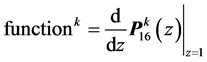
In order to determine the WCET, we have to differentiate the solution for the final node  with respect to z and after that set
 .
.
Let  refer to the function representing the solution of the kth component of the final node
 . According to well-known facts of generating functions [6] it is defined as

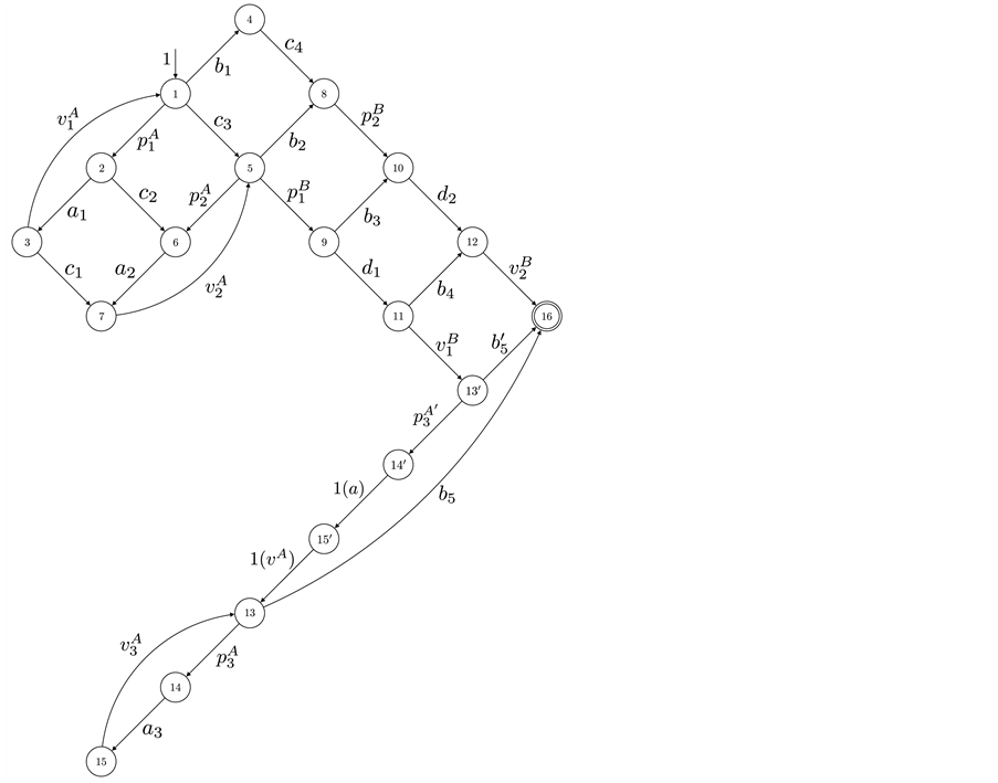
Figure 4. Adapted RCPG.
In order to calculate the loop iteration count for all loop copies and to calculate the undefined execution frequencies within the given constraints, we maximize this function. This goes beyond the approaches given in [4] [6] . During this maximization step, for which we used NMaximize of MathematicaÓ, e.g. all  are treated as variables. For each of these variables, Mathematica finds values within the given constraints. Thus, Mathematica assigns valid values for all
  and all the unknown execution frequencies. Of course, instead of Mathematica, any non-linear function solver capable of handling constraints can be used. The WCET of the kth CPU core is given by

In the following, the variable configuration found during this maximization is used. The WCET of a concurrent program consisting of n threads is defined as
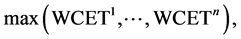
where the max is the ordinary maximum operator for numbers.
If the RCPG contains s vp-synchronizing nodes, then the maximization process has to be done  times. One time for each possible value of
  originating from the vp-synchronizing nodes. At last the largest value of those
  results represents the WCET of the concurrent program. Hence, the computational complexity may increase exponentially in s. Anyhow, s is usually small. For n threads and r semaphores, the
number of vp-synchronizing nodes in the CPG is bounded above by , where
  is the
number of v-operations of semaphore j in thread i and  is the number of p-operations of semaphore j in thread k. Depending on how the semaphores are used not all vp-synchronizing nodes may be part of the RCPG. In addition, information may be available which allows to conclude that even some of the present cases cannot result in the final WCET value. Then, these cases need not be considered in the maximization process. In [19] an example with CPG matrix size of 298721280 has been analyzed within 400 ms. It contained 13 semaphores and only 15 synchronization nodes. Even though the CPGs for travel time analysis do not contain loops, the number of synchronizing nodes is comparable.
5. Example
This small example includes synchronization and one single loop. We use two threads, namely A and B, sharing one single semaphore with the operations p and v. The CFGs of the two threads are depicted in Figure 1(b) and Figure 1(c). Each edge is labeled by a basic block l. Together with a RCFG of a binary semaphore, we calculate the adjacency matrix P of the corresponding RCPG in the following steps: The interleaved threads are given by
 Because we have only one semaphore, the interleaved semaphores are trivially defined as
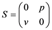 . The program’s matrix P is given by
 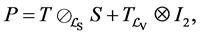 where
where  and
and . The
. The
RCPG of the A-B-system is depicted in Figure 3. The edges for the RCPG are labeled by their execution frequencies on RCPG level. Anyway, we indicate for each execution frequency  that it is the execution frequency for the x-th copy of basic block l.6
We assume that both threads access shared variables in the basic blocks a and d. Thus, the basic blocks a and d are only allowed to be executed in a mutually exclusive fashion. This is ensured by using a semaphore. The basic blocks a and d are protected by p-calls. After the corresponding thread finishes the execution of a or d, the semaphore is released by a v-call. We assume that all the other basic blocks do not access shared variables. Note that the threads are mapped to distinct processors and that these mappings are immutable.
Each variable x in this example (except ,
,  ,
,  and
and ) is a rational number such that
 . We assume that thread A's loop is executed
  times and the three copies of the loop are executed
 ,
,  and
and  times, respectively. Hence, we have the loop iteration constraint
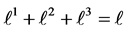 , where
 .
.
5.1. Equations Not Affected by Partial Loop Unrolling
Following the rules of Section 3, we obtain the following equations.
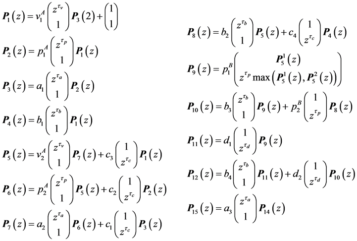
Note again that the max-operators in  and
and  (stated in Subsection 5.2) originate because the
original nodes 9 and 14, respectively, are vp-synchronizing nodes and that max is not the ordinary maximum operation using numbers as input. During the maximization process, for each max -operator we do the whole calculation twice, once for each possible solution.
5.2. Partial Loop Unrolling
Node 13 is a vp-synchronizing node and edge  constitutes a loop entry edge. Thus, we have to apply partial loop unrolling.
The changes in the equations can be interpreted on RCPG-level as depicted in Figure 4 (compare to Figure 3). For edges whose execution frequency is 1 we write 1(a) in order to state that the edge refers to the basic block a. For these edges, the execution time would otherwise be unclear. In the following, we use the Kronecker delta function. Kronecker delta  is defined as
By partially unrolling the loop, we get the execution frequencies:
 ,
,  ,
, 
Note that the non-linear function solver employed for the maximization process must be able to handle  and case functions (like that used in the right hand side of
 ) correctly.
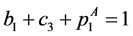
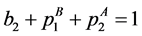
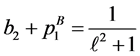
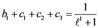
5.3. Execution Frequencies and Constraints
The following execution frequencies and constraints are extracted out of the RCPG. The execution frequencies of the loop entry edges  and
and  are established as follows:
 ,
, .
.
From the node constraints, we get ,
,  ,
,  ,
,  ,
,  ,
,  ,
,  and
and  statically set to 1. The remaining node constraints contribute execution frequency variables and the corresponding constraints for the final maximization process.
 ,
,  ,
,  ,
,  ,
,  ,
,  ,
, .
.
The loop exit constraints are as follows:
 ,
, .
.
The time needed for executing basic block b is referred to as . We assume that all copies of a certain basic block lead to the same execution time. Thus, e.g., each one out of
 ,
,  and
and  has an execution time of
 . Finally, for node 5, which is a pp-synchronizing node, we have the following constraints. These conditions follow from our computational model described in Section 2 and the fairness constraints from Subsection 4.3:
• ,
,
• ,
,
• .
.
5.4. Solving the Equations
For a concise presentation, we use the notation . We used two approaches to solve the equations. At first, we applied [20] . To double-check the solution, we used MathematicaÓ, too.
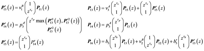
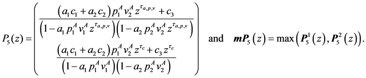
The resulting equations for the final node 16 are:
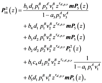
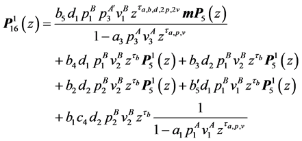
where
5.5. Maximization Process
Finally, we have to differentiate  with respect to z and then set
 .
.

where the set constraints consists of the constraints set up in Section 5.3. The WCET of the concurrent program consisting of two threads is defined by

In Table 1 some WCET values of the program and its components, namely the threads A and B, are depicted. The time needed for executing basic block b is referred to as . We assume that all copies of a certain basic block lead to the same execution time. Further we set
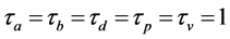 ,
,  , and let
  range from 1 to 10. As described above, during the maximization process, we let MathematicaÓ choose the values of the variables
  and all the unknown execution frequencies. We used the execution time
  as an input parameter to see how it affects the WCET of the program. Note that the calculated values are exact WCET values. In the rightmost column of Table 1, we present the average time needed by Mathematica to calculate the time of the component leading to the WCET. Note that the maximization dominates the overall CPU time. Generating the RCPG and solving the data flow equations takes only a few milli seconds. Mathematica 10 was executed on a CentOS 6.0, Intel Core i7 870 CPU, 2.96 GHz, 8 MB cache and 4GB RAM. Until now, our focus was not on using specialized non-linear solvers which would probably lead to much better maximization times. Finding the best non-linear function solver is ongoing research.
6. Related Work
Our approach is the first one capable of handling parallel and concurrent software. There exist several approaches for parallel systems which we will discuss in the following (see e.g. [21] for an overview).
In [7] an IPET based approach is presented. Communication between code regions in form of message passing is detected via source code annotations specifying the recipient and the latency of the communication. For each communication between code regions, the corresponding CFGs are connected via an additional edge. Hence, the data structure are CFGs connected via communication edges. This is not enough for programs containing recurring communication between threads. In contrast to that, our approach generates a new data structure (RCPG) out of the input CFGs in a fully automated way. The RCPG incorporates thread synchronization of

Table 1. WCET for  and multiple values of
 .
.
the multi-threaded program and thus contains only the reachable interleavings. Our approach is not limited to one single synchronization mechanism, it can be used to model e.g. semaphores or locks. In addition, RCPGs play a similar role for multi-threaded programs as CFGs do for sequential programs and can be used for further analysis purposes. The hardware analysis on basic block level of [7] can be applied to our approach too.
As our approach for loops, the work presented in [2] also relies on annotations. The worst case stalling time is estimated for each synchronization operation. This time is added to the time of the corresponding basic block. Our approach exactly detects the points where stalling will occur, i.e., at the vp-synchronizing nodes, and establishes dataflow equations to handle that problem in an explicit and natural way. It calculates the stalling times which need not be given by the user. At these points (e.g. critical section protected via a semaphore), we can also incorporate hardware penalties for all kinds of external communication and optimizations for e.g. shared data caches. Our approach allows synchronization within loops in a concurrent program whereas [2] does not support that. This is the main reason why [2] can use an ILP approach. Similar to [2] , we use a rather abstract view of synchronization primitives and assume timing predictability on the hardware level as discussed e.g. in [22] .
Current steps towards multi-core analysis including hardware modelling try to restrict interleavings and use a rigorous bus protocol (e.g. TDMA) that increases the predictability [23] . A worst-case resource usage bound to compute the WCET overlap is used. Hence, it finds a WCET upper bound only, while our approach determines the exact WCET that includes stalling times.
Since the model-checking attempt in [24] has scalability problems the authors switched to the abstract execution approach of [25] . It allows to calculate safe approximations of the WCET of programs using threads, shared memory and locks. Locks are modeled in a spinlock-like fashion. The problem of nontermination is inherent in abstract execution. Thus, it is not guaranteed in [25] that the algorithm will terminate. This issue is only partly solved by setting timeouts.
7. Conclusion and Future Work
In this paper, we focused on calculating stalling times automatically in an exact WCET analysis of shared memory concurrent programs running on a multi-core architecture. The stress was on a formal definition of both, our graph model and the dataflow equations for timing analysis. This is the first approach suited for parallel and concurrent systems.
We established a generic graph model for multi-threaded programs. Thread synchronization is modeled by semaphores. Our graph representation of multi-threaded programs plays a similar role for concurrent programs as control flow graphs do for sequential programs. Thus, a suitable graph model for timing analysis of multi- threaded software has been set up. The graph model serves as a framework for WCET analysis of multi-threaded concurrent programs. The usefulness of our approach has been proved by a lazy implementation of our extended Kronecker algebra. The implementation is very memory-efficient and has been parallelized to exploit modern many-core hardware architectures. Currently there is work in progress for a GPGPU implementation generating RCPGs. The first results are very promising.
We applied a generating functions approach. Dataflow equations are set up. The WCET is calculated by a non-linear function solver. Non-linearity is inherent to the multi-threaded WCET problem. The reasons are that (1) several copies of loops show up in the RCPG and (2) partial loop unrolling has to be done in certain cases. (1) implies that loop iteration numbers for loop copies have to be considered variable until the maximization process takes place. Thus, nested loops cause non-linear constraints to be handed to the function solver. (2) generates additional non-linear constraints.
In terms of WCET analysis a lot of work remains to be done. The focus of this paper is on how to model concurrent programs. One future work may be modelling hardware features. In general, without taking into account e.g. pipelining, shared cache, shared bus, branch prediction and prefetching, we might overestimate the WCET. Our approach could benefit from e.g. [26] - [28] which support shared L2 instruction caches.
Finding the best non-linear function solver is ongoing research. MathematicaÓ was just the first attempt. This will probably lead to better maximization times. A direction of future work is to generalize for multiple threads running on one CPU core. We will investigate how an implicit path enumeration technique (IPET) approach [8] together with non-linear solvers can produce similar results to our approach. Finally, a possible direction for future work could be a WCET analysis of semaphore-based barrier implementations [5] .
Cite this paper
Robert Mittermayr,Johann Blieberger, (2016) A Generic Graph Model for WCET Analysis of Multi-Core Concurrent Applications. Journal of Software Engineering and Applications,09,182-198. doi: 10.4236/jsea.2016.95015
References
- 1. Wilhelm, R., Engblom, J., Ermedahl, A., Holsti, N., Thesing, S., Whalley, D., Bernat, G., Ferdinand, C., Heckmann, R., Mitra, T., Mueller, F., Puaut, I., Puschner, P., Staschulat, J. and Stenstrom, P. (2008) The Worst-Case Execution-Time Problem—Overview of Methods and Survey of Tools. ACM Transactions on Embedded Computing Systems, 7, Article No. 36.
http://dx.doi.org/10.1145/1347375.1347389 - 2. Ozaktas, H., Rochange, C. and Sainrat, P. (2013) Automatic WCET Analysis of Real-Time Parallel Applications. WCET 2013, 30, 11-20.
- 3. Buchholz, P. and Kemper, P. (2002) Efficient Computation and Representation of Large Reachability Sets for Composed Automata. Discrete Event Dynamic Systems, 12, 265-286.
http://dx.doi.org/10.1023/A:1015669415634 - 4. Mittermayr, R. and Blieberger, J. (2012) Timing Analysis of Concurrent Programs. WCET 2012, 23, 59-68.
- 5. Mittermayr, R. and Blieberger, J. (2016) Kronecker Algebra for Static Analysis of Barriers in Ada (to Appear). In: Bertogna, M., Pinho, L.M. and Quinones, E., Eds., 21st International Conference on Reliable Software Technologies, LNCS, Springer Press.
- 6. Blieberger, J. (2002) Data-Flow Frameworks for Worst-Case Execution Time Analysis. Real-Time Systems, 22, 183-227.
http://dx.doi.org/10.1023/A:1014535317056 - 7. Potop-Butucaru, D. and Puaut, I. (2013) Integrated Worst-Case Execution Time Estimation of Multicore Applications. WCET 2013, 30, 21-31.
- 8. Puschner, P. and Schedl, A. (1997) Computing Maximum Task Execution Times—A Graph-Based Approach. Journal of Real-Time Systems, 13, 67-91.
http://dx.doi.org/10.1023/A:1007905003094 - 9. Tarjan, R.E. (1981) A Unified Approach to Path Problems. Journal of the ACM, 28, 577-593.
http://dx.doi.org/10.1145/322261.322272 - 10. Stallings, W. (2011) Operating Systems—Internals and Design Principles. 7th Edition, Prentice Hall, Upper Saddle River.
- 11. Aho, A., Sethi, R. and Ullman, J. (1986) Compilers: Principles, Techniques, and Tools. Addison Wesley, Massachusetts.
- 12. Mittermayr, R. and Blieberger, J. (2011) Shared Memory Concurrent System Verification Using Kronecker Algebra. Technical Report 183/1-155, Automation Systems Group, TU Vienna.
http://arxiv.org/abs/1109.5522 - 13. Davio, M. (1981) Kronecker Products and Shuffle Algebra. IEEE Transactions on Computers, 30, 116-125.
http://dx.doi.org/10.1109/TC.1981.6312174 - 14. Graham, A. (1981) Kronecker Products and Matrix Calculus with Applications. Ellis Horwood Ltd., New York.
- 15. Harary, F. and Trauth Jr., C.A. (1966) Connectedness of Products of Two Directed Graphs. SIAM Journal on Applied Mathematics, 14, 250-254.
http://dx.doi.org/10.1137/0114024 - 16. Küster, G. (1991) On the Hurwitz Product of Formal Power Series and Automata. Theoretical Computer Science, 83, 261-273.
http://dx.doi.org/10.1016/0304-3975(91)90278-A - 17. Burgstaller, B. and Blieberger, J. (2014) Kronecker Algebra for Static Analysis of Ada Programs with Protected Objects. In: George, L. and Vardanega, T., Eds., Reliable Software Technologies—Ada-Europe 2014, Springer International Publishing, New York, 27-42.
http://dx.doi.org/10.1007/978-3-319-08311-7_4 - 18. Kirner, R., Knoop, J., Prantl, A., Schordan, M. and Kadlec, A. (2011) Beyond Loop Bounds: Comparing Annotation Languages for Worst-Case Execution Time Analysis. Software & Systems Modeling, 10, 411-437.
http://dx.doi.org/10.1007/s10270-010-0161-0 - 19. Volcic, M., Blieberger, J. and Schobel, A. (2012) Kronecker Algebra Based Travel Time Analysis for Railway Systems. 9th Symposium on Formal Methods for Automation and Safety in Railway and Automotive Systems, Braunschweig, 12-13 December 2012, 273-281.
- 20. Sreedhar, V.C., Gao, G.R. and Lee, Y.-F. (1998) A New Framework for Elimination-Based Data Flow Analysis Using DJ Graphs. ACM Transactions on Programming Languages and Systems, 20, 388-435.
http://dx.doi.org/10.1145/276393.278523 - 21. Axer, P., Ernst, R., Falk, H., Girault, A., Grund, D., Guan, N., Jonsson, B., Marwedel, P., Reineke, J., Rochange, C., Sebastian, M., Von Hanxleden, R., Wilhelm, R. and Wang, Y. (2014) Building Timing Predictable Embedded Systems. ACM Transactions on Embedded Computing Systems, 13, Article No. 82.
http://dx.doi.org/10.1145/2560033 - 22. Gerdes, M., Kluge, F., Ungerer, T. and Rochange, C. (2012) The Split-Phase Synchronisation Technique: Reducing the Pessimism in the WCET Analysis of Parallelised Hard Real-Time Programs. IEEE International Conference on Embedded and Real-Time Computing Systems and Applications, Seoul, 19-22 August 2012, 88-97.
http://dx.doi.org/10.1109/rtcsa.2012.11 - 23. Nowotsch, J., Paulitsch, M., Buhler, D., Theiling, H., Wegener, S. and Schmidt, M. (2014) Multi-Core Interference-Sensitive WCET Analysis Leveraging Runtime Resource Capacity Enforcement. 26th Euromicro Conference on Real-Time Systems, Madrid, 8-11 July 2014, 109-118.
http://dx.doi.org/10.1109/ecrts.2014.20 - 24. Gustavsson, A., Ermedahl, A., Lisper, B. and Pettersson, P. (2010) Towards WCET Analysis of Multicore Architectures Using UPPAAL. 10th International Workshop on Worst-Case Execution Time Analysis, Brussels, 6 July 2010, 101-112.
- 25. Gustavsson, A., Gustafsson, J. and Lisper, B. (2014) Timing Analysis of Parallel Software Using Abstract Execution. In: McMillan, K.L. and Rival, X., Eds., Lecture Notes in Computer Science, Springer, Berlin, 59-77.
http://dx.doi.org/10.1007/978-3-642-54013-4_4 - 26. Chattopadhyay, S., Chong, L.K., Roychoudhury, A., Kelter, T., Marwedel, P. and Falk, H. (2012) A Unified WCET Analysis Framework for Multi-Core Platforms. IEEE 18th Real Time and Embedded Technology and Applications Symposium, Beijing, 16-19 April 2012, 99-108.
http://dx.doi.org/10.1109/rtas.2012.26 - 27. Liang, Y., Ding, H.P., Mitra, T., Roychoudhury, A., Li, Y. and Suhendra, V. (2012) Timing Analysis of Concurrent Programs Running on Shared Cache Multi-Cores. Real-Time Systems, 48, 638-680.
http://dx.doi.org/10.1007/s11241-012-9160-2 - 28. Yan, J. and Zhang, W. (2008) WCET Analysis for Multi-Core Processors with Shared L2 Instruction Caches. IEEE Real-Time and Embedded Technology and Applications Symposium, St. Louis, 22-24 April 2008, 80-89.
http://dx.doi.org/10.1109/rtas.2008.6
NOTES

1These execution times do not include stalling time which we calculate automatically.

2A k-by-k matrix is known as square matrix of order k.

3For simplicity, we chose constant; our approach supports upper bounds too.
4According to the definition of vp-synchronizing nodes .
.
5Note that we can detect these nodes when generating the RCPG.

6A hardware analysis may detect that the copies of a basic block have different execution times due to e.g. shared data caches or instruction pipelining.