Journal of Software Engineering and Applications
Vol. 5 No. 3 (2012) , Article ID: 18291 , 10 pages DOI:10.4236/jsea.2012.53020
Visualization of Pareto Solutions by Spherical Self-Organizing Map and It’s Acceleration on a GPU
![]()
1Factuly of Engineering, Doshisha University, Kyoto, Japan; 2Faculty of Department of Life and Medical Science, Doshisha University, Kyoto, Japan.
Email: myoshimi@mikilab.doshisha.ac.jp
Received February 1st, 2012; revised March 1st, 2012; accepted March 12th, 2012
Keywords: Self-Organizing Map; SOM; Spherical; GPU; Pareto-Optimal Solutions; GPU Acceleration
ABSTRACT
In this study, we visualize Pareto-optimum solutions derived from multiple-objective optimization using spherical self-organizing maps (SOMs) that lay out SOM data in three dimensions. There have been a wide range of studies involving plane SOMs where Pareto-optimal solutions are mapped to a plane. However, plane SOMs have an issue that similar data differing in a few specific variables are often placed at far ends of the map, compromising intuitiveness of the visualization. We show in this study that spherical SOMs allow us to find similarities in data otherwise undetectable with plane SOMs. We also implement and evaluate the performance using parallel sphere processing with several GPU environments.
1. Introduction
With the rapid rise of hardware and software performance in recent years, computer-aided numerical simulations are being used more and more for designing products. These include construction drawings with CAD (Computer-Aided Design), optimizations of design parameters, and validations of candidate solutions, among others.
It is often effective to formalize problems as optimization problems in order to employ numerical simulations as design aids. An optimization problem is one in which design variables are determined so that one or more objective functions yield the highest or lowest possible values under certain conditions. Real-world optimization problems tend to have multiple objective functions that pose trade-offs among each other: this type of problem is called a multiple-objective optimization problem. Because of the trade-offs, a multiple-objective optimization problem has multiple optimal points, each of which is the most fit for a certain objective function. The set of these solutions is called the Pareto-optimal solution set. Many approaches have been proposed on how to reach the Pareto-optimal solution set [1].
In product design, an important task is to choose the best solutions from a Pareto-optimal solution set. It is required, then, to visualize the solution set and show the designer what characteristics each of the solutions have in relation to other solutions and in relation to the containing set. However, whereas each solution in a multipleobjective optimization problem is a multi dimensional value consisting of many objective function values and design variables, the human eye can distinguish and comprehend merely three dimensions at most. This gap needs to be bridged in order to present an intuitive visualization.
One attempt at this challenge is the self-organizing map (SOM) [2], a kind of artificial neural network. A SOM is a means of translating high-dimension data to low-dimension data and is useful for visualizing a Paretooptimal solution set, typically in three or less dimensions.
Meanwhile, practical use of data analysis on the job site demands short execution times. Although future improvements in hardware performance will allow larger and larger problems to be computed in realistic timeframes, thus enabling a wider range of design aids, recent years have seen the increase of processor frequency hit the ceiling. Instead, grounds for performance gains are shifting to many-core architectures, namely graphic processing units (GPUs). Many-core architectures have multiple processing cores and yield exceptionally good performance with parallel algorithms. Thus, when handling large problems, one should employ highly parallel algorithms that are computed faster with many-core architectures.
While SOMs require a vast amount of computations, they also have high loop-level parallelism and can be expected to perform well on many core architectures [3].
Based on these premises, we explored the visualization of Pareto-optimal solutions using SOMs (spherical SOMs [4] specifically) and evaluated the system using a GPUbased implementations. Spherical SOMs have been reported [5] to be less vulnerable to distortions compared to plane SOMs due to the fact that they have no edges. They also show a comparatively rational spatial relationship among the data points and can be clustered more accurately [4,6].
In this paper, we discuss first the parallelizing of the spherical SOM algorithm, then evaluate its performance with a GPU-based implementation. Subsequently we discuss the visualization of Pareto-optimal solution sets for two optimization problems: test functions commonly used in multi-objective genetic algorithms, and a problem concerning the design of diesel engines, thus pointing out the effectiveness of spherical SOMs and their advantages over planar SOMs.
2. Multi-objective Optimization Problems
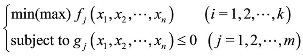
A problem where multiple objectives must be optimized at the same time is called a multi-objective optimization problem. A multi-objective problem is generally formalized as Equation (1): there are n design variables x, and k objective functions f(x) are maximized (or minimized) under m constraints g(x).
 (1)
(1)
Because it is often the case with multiple-objective optimization that there are trade-offs among objective functions, not all objective functions  can be optimized at the same time. Therefore we aim for a set of Paretooptimal solutions rather than a single optimal solution. Pareto-optimal solutions are defined by the solutions’ dominance over each other. Below is the definition of dominant solutions in multiple-objective optimization problems (when all objective functions are optimal when minimized):
Definition of dominance:
When (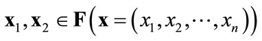 )
)
(a)  dominates
  when
when
(b)  strongly dominates
  when
when

A solution  that dominates
  is better than
  in the general sense. The intent then is to search for nondominated solutions. Based on this definition of dominance, below is the definition of Pareto-optimal solutions:
Definition of Pareto-optimal solutions:
When ( )
)
(a)  is a weak Pareto-optimal solution when there are no solutions
  that strongly dominate
(b)  is a Pareto-optimal solution when there are no solutions
  that dominate
Figure 1 shows an example of Pareto-optimal solutions when there are two objectives (k = 2). Solid dots show Pareto-optimal solutions. Open dots are inferior in every way to Pareto-optimal solutions. Thus we can ignore the white dots and obtain the front consisting of Pareto-optimal solutions, which is shown as the dashed curve (the Pareto-optimal front).
One way to visually investigate what kinds of Paretooptimal solutions constitute a Pareto-optimal solution set is SOM.
3. SOM
3.1. SOM Overview
SOM is a type of neural network trained by unsupervised learning and is known as a means of data mining. SOM can map a group of data into an arbitrary number of dimensions without distorting correlations among these data points. Thus it is useful for visualizing high dimension data into lower dimensions (typically two or three) so that characteristics can be grasped intuitively. It also lets us cluster the solution set and analyze its traits.
3.2. SOM Algorithm
A SOM consists of two layers: the competitive layer and the input layer. The competitive layer is where neurons are placed, and the input layer is the group of input data points. Neurons on the competitive layer are updated as the SOM is trained with successive read-ins from the input layer.
An input data point, defined as , is presented to all neurons in the network. Any given neuron i has a weight vector with number of dimensions n, corresponding to the dimensions of the input data. A neuron’s weight vector for a given time t is defined as
 . Learning coefficient α(t), neighborhood function hci(t), and neighborhood range σ(t) are also defined. A basic SOM algorithm is as follows:
1) Initialize competitive layer With  and the repetition count
 , all neurons
  in the competitive layer are set with initial weight vectors.
2) Compute distances Input data point  is presented to the competition layer and Euclidian distances from the neurons
 are computed.
3) Find the winner neuron The winner neuron c where
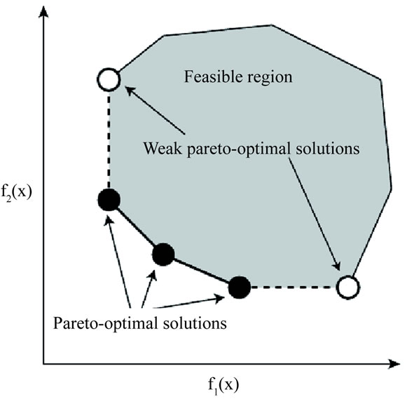
Figure 1. Pareto-optimum solutions.
 is determined.
4) Train The winner neuron c and all neurons within distance dci from it are adjusted by applying Equations (2). The neighborhood function hci(t) is defined by Equations (3) using the learning coefficient α(t). α(t) and the neighborhood range σ(t) are defined by Equations (4) and (5) respectively.
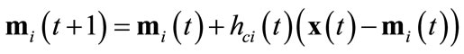 (2)
(2)
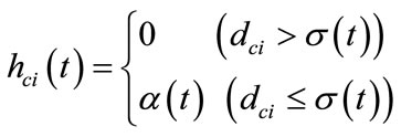 (3)
(3)
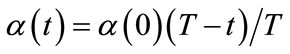 (4)
(4)
 (5)
(5)
5) Terminate If , set
, set  and return to step (2). Otherwise exit the loop.
4. Spherical SOM
4.1. Spherical SOM Overview
When analyzing a Pareto-optimal solution set, it is important not only to grasp where the solutions are clustered, but also to see what other neighboring solutions exist for a given solution, or how the solutions are positioned in relation to each other.
A map generated with SOM shows similar data points close to each other, which is helpful in assessing the similarities of the solutions. However, the fact that a pair of data points is placed far from each other on the map does not necessarily mean that the similarity is low. A designer analyzing a Pareto-optimal solution set would prefer similar data points to appear as close to each other on the map as possible.
This apparent similarity (or proximity) of the solutions depends heavily on the form of the competitive layer used in SOM. A competitive layer in the shape of a twodimensional plane often yields distortions in proximity because edges exist, and the number of neurons in the neighborhood range differs from neuron to neuron. To avoid this, SOMs with competitive layers in closed forms such as tori or spheres have been proposed.
Torus SOMs are easy to implement as an extension to plane SOMs, but the resulting visualization takes the form of a donut, which is difficult to interpret with human eyes, whereas spherical SOMs place the neurons on the surface of a sphere, making it easier to grasp the spatial relations. Thus spherical SOMs are suitable for visualization.
4.2. Implementation of a Spherical SOM
4.2.1. Data Structure
Neurons in a spherical SOM are commonly placed in a geodesic dome, a type of quasi-regular polyhedron [5]. A geodesic dome is an approximated sphere constructed by halving each edge of a regular polyhedron, thus recursively increasing the number of surfaces. Neurons are placed on the apices of the geodesic dome, forming a hexagonal grid. Apices on a geodesic dome give the neurons a more uniform arrangement on the surface of a sphere compared to other methods such as polar coordinates. In this study we used a regular icosahedron, the regular polyhedron with the largest possible number of surfaces, for the original approximation of the sphere to further ensure uniformity.
A geodesic dome, when unfolded via the edges of the icosahedron, forms a net that can be mapped to and handled in two dimensions. Thus, our competitive layer is represented as a two-dimensional array of neurons as shown in Figure 2.
4.2.2. Parameters of the Neuron Struct
The neurons in the two-dimensional array mentioned above have a data structure with the following properties:
List of links to adjacent neurons There are 6 adjacent neurons for any given neuron, for they are placed on a hexagonal grid. Array indices for adjacent neurons can be computed using a fairly simple function for a plane SOM, but are unable to compute in some cases for a spherical SOM, namely at the edges of the net. Therefore we store the addresses of the adjacent neurons as a list for later reference.
Weight vector The weight vector is stored as a one-dimensional array.
Euclid distance This property temporarily holds the computed distance between a neuron and a given input data point.
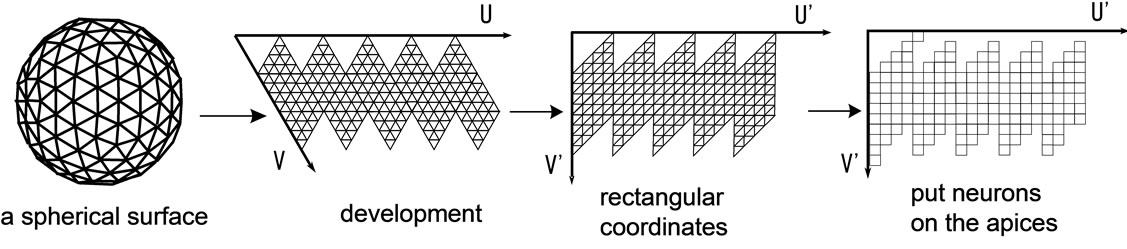
Figure 2. Description of spherical surface on a two-dimensional array.
Trained flag This flag is turned on if a neuron has already been trained with a given input data point to avoid redundant exposures.
Validity flag This flag is turned off if a neuron is not a valid part of competitive layer, in which case it should be excluded when computing distances and winner neurons.
Three-dimensional coordinates These coordinates are used to draw a three dimensional sphere.
4.2.3. Distance and Winner Neuron Computation
Because the neurons are placed in a two-dimensional array, distances and BMUs can be computed by simply scanning this array, as with a plane SOM. They are filtered before computation, however, according to their validity flags.
4.2.4. Choosing Neurons to Be Trained
A SOM is trained by choosing neurons that are within a certain distance from a given point and adjusting them. In order to choose these neurons, we construct a search tree that has a certain depth by recurring into the link of adjacent neurons, thus representing a range of neurons to be trained. The tree is then traversed breadth first so that neurons closer to the origin (winner neuron) are trained first. Below are the details of this process.
First, the winner neuron is trained. Then, we retrieve all adjacent neurons of the winner neurons and train them. At the same time, a list of neurons trained is created as shown in Figure 3. Then, we train the neurons that are adjacent to the ones in the list, effectively moving outward (these neurons are also stored in a new list).
The trained flag is checked before each neuron is trained so that one neuron does not get trained multiple times from one input data point. Thus we recursively train neighboring neurons of the winner without duplications or omissions.
4.2.5. Displaying the Competitive Layer
It is often effective to colorize each neuron when displaying the competitive layer as a visualization. We mapped the weight vector of each of the neurons into the HSV color space to colorize the neurons. The Saturation and Value were fixed to the maximum, while the Hue was determined from the weight vector. The Hue can take any value in range [0, 360]. We used values in range [0, 280] so that large values show up as red and small values show up as purple.
5. Execution of Spherical SOM with GPUs
5.1. Hardware Acceleration
The SOM algorithm is known to have high parallelism for its distance computation, winning neuron computation, and training in each cycle of its execution. Therefore we can expect fast execution using recent technologies such as multi-core processors and other hardware suitable for parallel computation.
High-speed executions of SOMs have been much debated since the well-known research by Carpenter, et al. on hardware acceleration in 1987 [7]. COKOS (Coprocessor for Kohonen’s Self-organizing map), a SIMD processor specifically for SOMs, was developed by Speckman in 1992 [8]. This processor had 8 parallel processing cores and was designed to make the most out of SOM’s parallelism.
There have also been attempts to construct a SOM accelerator on FPGA by Porrmann and Tamukoh [9]. Porrman constructed a piece of hardware that executes SOMs with 6 processing modules connected to each other in a ring topology. Tamukoh implemented a piece of hardware that chooses a winner neuron by computing all distances at once and evaluated it using a vector dimension number of 128 and a map size of 16 by 16. He also used Manhattan distances instead of Euclidian distances to simplify computations and reduce circuit size. Processing modules and data memories existed for each weight vector, and the way these modules connected with each other replicated the competitive layer. Thus the modules were able to compute in a massively parallel manner. This piece of hardware could compute a SOM in constant time regardless of map size, and was proved to be 350 times faster than an Intel Xeon 2.80 GHz CPU.
In 2009 Shitara attempted a high-speed execution of SOM using a GPU. He used an NVIDIA GeForce GTX- 280, which was 150 times faster than a CPU [10]. This high parallelism holds for spherical SOMs as well. In this study we use GPUs for which development environments

Figure 3. Choosing neurons to be trained.
have been published (and are actively researched) to implement a spherical SOM and discuss the performance based on execution with GPUs and conventional CPUs.
5.2. Parallelizing the SOM Algorithm
Let us discuss which parts of the SOM algorithm may be parallelized.
The most costly process in the algorithm is the computations of Euclidian distances between input vectors and neurons’ weight vectors. These computations are independent from each other so they may be parallelized.
Selecting the winner neuron, the process in which a neuron with the minimum Euclidian distance is determined, may also be parallelized. Sequential comparison would be O(n), but this can be reduced to O(log(n)) by employing a tournament-style comparison with binary trees.
Training of the neurons may also be parallelized. In this process, computations against weight vectors for all neurons within a certain distance from the winner neuron are to be performed for a given input data point. These adjustments are independent of each other and may be parallelized.
5.3. Evaluation
Based on the above facts, we implemented a spherical SOM program that is executable with a GPU, and evaluated its execution speed.
C++, along with CUDA, NVIDIA’s GPU development environment, was used in implementation. The GPUs we used are 1) GeForce 8400GS, 2) GeForce GTX280, and 3) Tesla C1060. Table 1 shows their technical specifications.
We also implemented a spherical SOM program for CPU to compare. The CPU we used was 4) Opteron 1210 HE.
SOM settings were as follows:
• 5-dimensional neurons
• 50,000 (20 × 502) weight vectors
• [0,9] neighborhood range
5.3.1. Results
Table 2 shows execution times for each GPU and CPU.

Table 1. Technical specification for each GPU and CPU.
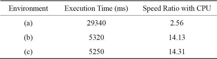
Table 2. Execution times for each GPU and CPU.
The results show that GPU acceleration is effective with spherical SOMs just as it is with plane SOMs. Figure 4 shows execution times for each of the steps in the SOM algorithm. Figure 5 shows percentages of time taken for each step for each processor.
5.3.2. Discussions
Tables 1 and 2 show that the two processors with the most SPs (stream processors) performed more than 10 times better than the CPU. This is due to the fact that performance gain is nearly proportional to the number of SPs when parallelism is high.
Figures 4 and 5 show that the proportion of distance calculation time is high with the 8400 GS. This is apparently because we passed the input neuron as an argument to the GPU function. The size of data passed results in (the number of calls x number of input neurons), which is considerably large. The 8400GS has a low memory bandwidth compared to the other GPUs and thus could not handle the computations as swiftly.
Figure 5 shows that parallelizing was especially effective with distance calculations. Although the 8400 GS (which has relatively few SPs and a lower frequency) took more time than CPU, the GPUs with 240 SPs were more than 10 times faster than CPU. On the other hand, winner selection and training have lower parallelisms than distance calculation.
Compared to plane SOM in research [10], we have a lower rate of acceleration for spherical SOM. This is a result of the way adjacent neurons are accessed. We used a list of links to access adjacent neurons of a certain neuron. Thus we must dereference the link every time we access an adjacent neuron, and this results in considerably more memory accesses, rendering parallelization less effective.
This problem may be solved by the use of Fermi. Fermi is a GPU architecture for GPGPUs developed by NVIDIA. One of the advantages over conventional GPUs is its memory access speed, which was improved by in-
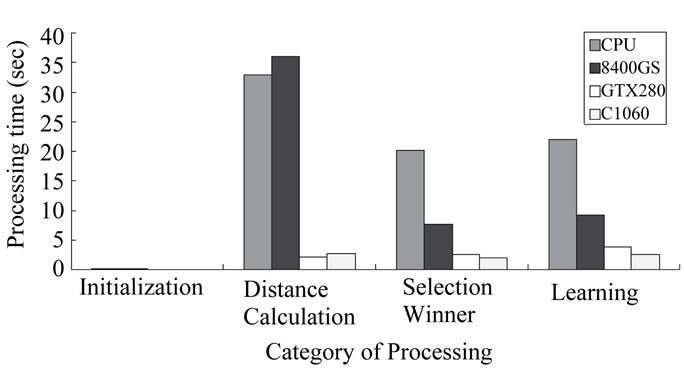
Figure 4. Execution time of each operation on each environment.

Figure 5. Percentage of execution time on each operation.
stalling a cache memory. Reduction of memory access overhead using Fermi shall result in a better parallel acceleration of spherical SOM.
6. Visualizing Pareto-Optimal Solutions with Spherical SOM
6.1. Spherical SOM with a Test Function
In this section we discuss how a Pareto-optimal solution set may be visualized by spherical SOM. First we shall engage ZDT2, a common test function for multi-objective optimization problems. ZDT2 is a monomodal and non-convex function defined by Expression (6).
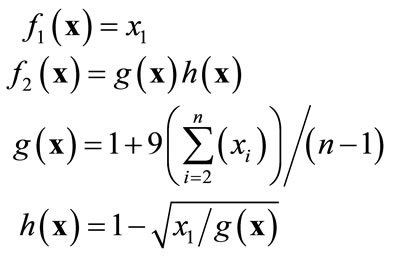 (6)
(6)
Using spherical SOM, we visualized data containing objective functions for Pareto-optimal solutions obtained from ZDT2 and the design parameters that determined them. The input data consisted of 12 dimensions: 2 dimensions of objective functions  and 10 dimensions of design variables
 . We used 100 data points.
For comparison we used SOMPAK, a freely available plane SOM program package. SOMPAK allows us to configure the dimensions of the competitive layer, amongst others, and can output the training results in both numeric and image formats. For this experiment we configured the lattice to a hexagonal grid and the neighborhood function to a step function. Table 3 shows the other configurations. Also, we set the initial number of exposures to 100,000, meaning the 100 Pareto-optimal solutions would be exposed to the competitive layer 1,000 times each.
To meet the conditions of the plane SOM, our spherecal SOM was configured with a step function as the neighborhood function. The competitive layer was initialized with random values. Table 3 shows configurations for the spherical SOM as well.
Figure 6 is the result from the plane SOM. It is colored with the same method as the spherical SOM. It shows that high values for  concentrate on the lower right corner and low values for
  concentrate on the lower left corner.
Figure 8 shows the parameters represented by points ,
,  and
and  on Figure 7. From these parameters alone, these three data points are similar in pattern.
  and
and , particularly, should be placed rather close to each other on the visualized map.
Of course, this is not to say that all similar data points appeared close to each other on the spherical SOM. However, we have shown that some relationships other-
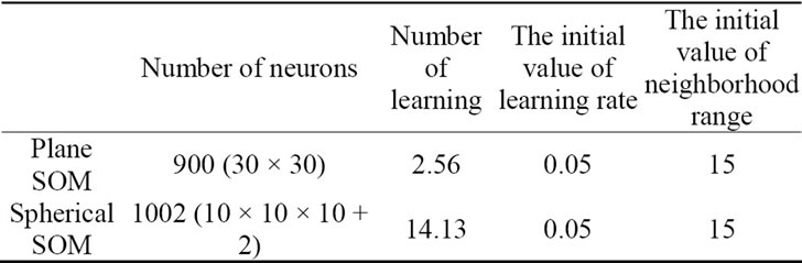
Table 3. Configurations of the SOM.

Figure 6. Visualization of ZDT2 on a spherical SOM.

Figure 7. Visualization of ZDT2 by plane SOM.

Figure 8. Objective functions and design variables for each points (p1, p2, p3).
wise obscured in the plane SOM were indeed observable in the spherical SOM.
The next section shall describe how the same is true for a diesel engine design problem.
6.2. Fuel Injection Scheduling for Diesel Engines
6.2.1. Overview
Diesel engines are generally more durable and fuel-efficient than gasoline engines, and they also have a lower CO2 emission. However, ecological concerns are rising and regulations have become more strict. In reacengines’ CO2 emission, gasoline and diesel alike.
Recent diesel engines make it possible to electronically control the EGR rate (exhaust gas recirculation rate) and swirl ratio. Timings of fuel injection and its chronological ratios can also be altered. Modifying these values have the effect of changing the SFC (specific fuel consumption) and the amount of NOx (nitrogen oxides) generated. Attempts have been made to electronically control engine parameters to reduce SFC, NOx emission and soot emission at once. This optimization problem is called the diesel engine fuel injection scheduling problem, and is usually handled as a multiple-objective optimization problem because there are trade-offs between NOx and soot as well as NOx and SFC.
In this experiment we deal with two-stage fuel in jections, as shown in Figure 9. The design variables are the parameters of a diesel engine that are electronically controllable now or will be controllable in the future, including the boost pressure, EGR rate, start angle, and swirl ratio. Table 4 shows the 11-dimensional data used for this experiment. The design variables are as they appear in paper [11].
Pareto-optimal solutions with different SFC, NOx and soot values can be obtained by adjusting the design variables. This experiment used data that contains the 3 dimensions of objective functions and 8 dimensions of design variables.
6.2.2. Visualization of the Pareto-Optimal Solution Set Using Spherical SOM
We trained a spherical SOM 1000 times using 100 Pareto-optimal solutions obtained from the fuel injection
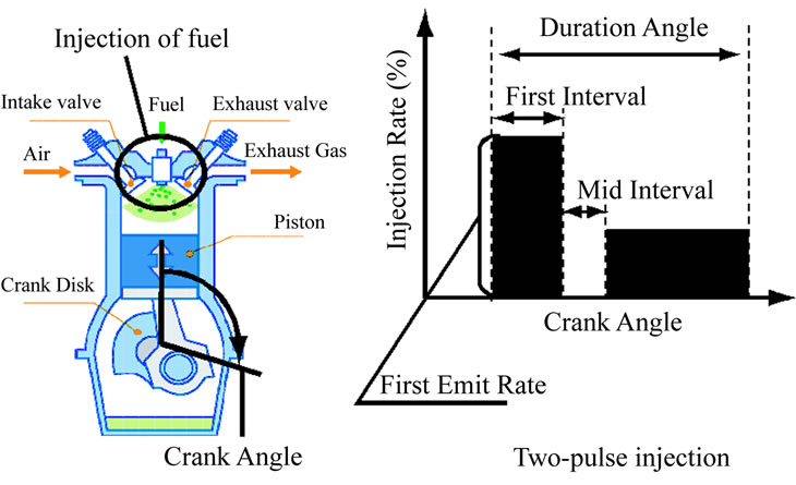
Figure 9. Injection mechanism of diesel.
scheduling problem. Configurations for SOMPAK and the spherical SOM were identical to those shown in Table 3.
Figure 10 shows results from the spherical SOM. Each sphere in these images is turned to the left by 90 degrees to render the next one. The sphere is colored according to SFC values: red when SFC is high and purple when low. A cluster of red is shown where SFC is particularly high.
Figure 11 shows the visualization by plane SOM. High SFC values are concentrated to the top left, and the values go down in the order of top right corner, bottom right corner and bottom left corner.
Both the spherical SOM and plane SOM show SFC values change gradually as we move from one point to another. Thus the spherical SOM is capable of categorizing and visualizing the solution space, just as Obayashi [12] stated was possible for plane SOM.
6.2.3. Differences in Data Placement
We have seen that plane SOM can effectively visualize a Pareto-optimal solution set, but some data that are similar to each other may have been positioned on opposite edges. We shall investigate where points of data from plane SOM (Figure 11) are shown in spherical SOM.
First let us look at p2 and p4. The objective functions and design variables are relatively similar, and should be displayed close to each other in a SOM visualization. However, in the plane SOM, they are placed on opposite edges on the right side. This results in the data points 
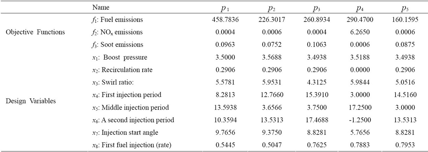
Table 4. Design variables and objective function of input data.
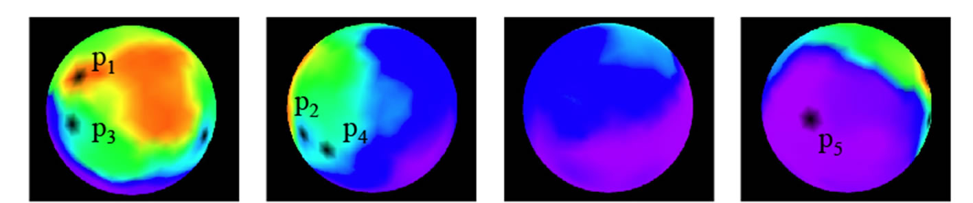
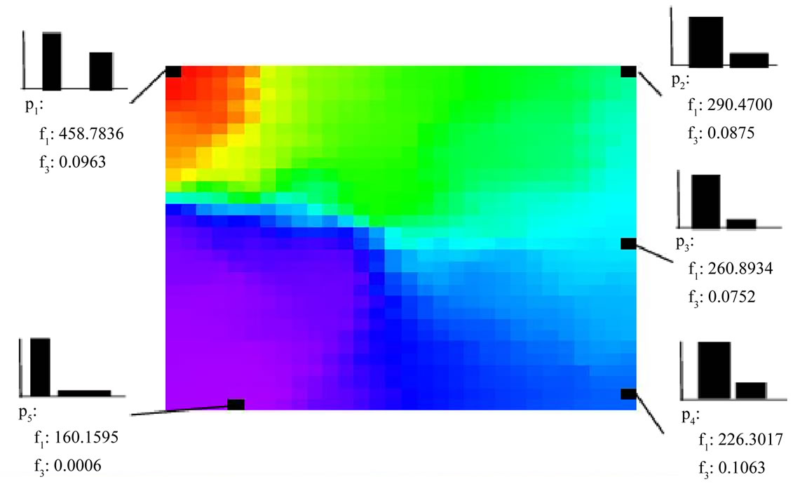
Figure 11. Visualization of SFC space on a plane SOM.
through  to be mapped to a sideways U-shape spanning over the entire map. On the other hand, the spherical SOM in Figure 10 shows
  and
and  side by side.
Next, let us look at  and
and . Because these injections differs in shape, as shown in Figure 11, the value of
  differs, and so does each point in Figure 10. However, whereas p1 and p3 are plotted far from each other in plane SOM (Figure 11), they are close by in spherical SOM (Figure 10). This is the result of design variables
  through
  in Table 4
  through
  determine the shape of injection. p1 and p3 have different values for these variables, but the other variables are similar. These points were seen as completely different on the plane SOM, but on the spherical SOM they are seen as similar points of data, albeit being in different clusters. This means that the spherical SOM was capable of a certain kind of clustering not offered by the plane SOM.
These results tell us that not only does the spherical SOM have the same benefits of the plane SOM, but can also present similarities more accurately. Thus the spherical SOM is suitable for visualizing a Pareto-optimal solution set.
7. Conclusions
In this study, we discussed the visualization of Paretooptimal solutions of multiple-objective optimization problems using SOMs (self-organizing maps). More specifically, we focused on spherical SOMs instead of the traditional plane SOMs. Plane SOMs can cause distortions of data along its edges, whereas spherical SOMs, due to the fact that they have no edges, can visualize similarities among data more accurately. We also implemented a spherical SOM for execution with GPUs and evaluated its performance.
First we described the details of implementation and discussed its parallelism. Then we compared its execution time with multiple GPUs and a CPU. The results showed that GPU usage yielded considerably higher performance.
Then we used two Pareto-optimal solution sets from multiple-objective optimization problems to evaluate the effectiveness of spherical SOMs. The first was a test function commonly used in research for multiple-objective optimization, and the other was a real-life diesel engine fuel injection scheduling problem. We showed from the results that the spherical SOMs not only offered the benefits of the plane SOM but also was capable of mapping data more accurately. We also showed that spherical SOMs let us grasp more versatile clusters of data. Thus, using a spherical SOM to visualize a Pareto-optimal solution set is a highly viable approach.
In future studies, we shall evaluate spherical SOMs and their implementations on a variety of problem sizes. We shall also further validate the use of GPUs for spherical SOMs and, at the same time, make attempts to make memory access more efficient.
REFERENCES
- P. Czyzżak and A. Jaszkiewicz, “Pareto Simulated Annealing—A Metatheuristic Technique for Multiple-Objective Combinatorial Optimization,” Journal of Multi-Criteria Decision Analysis, Vol. 7, No. 7, 1998, pp. 34-47. doi:10.1002/(SICI)1099-1360(199801)7:1<34::AID-MCDA161>3.0.CO;2-6
- T. Kohonen, “The Self-Organizing Map,” Proceedings of the IEEE, Vol. 78, No. 9, 1990, pp. 1464-1480. doi:10.1109/5.58325
- R. D. Prabhu, “SOMGPU: An Unsupervised Pattern Classifier on Graphical Processing Unit,” IEEE Congress on Evolutionary Computation, IEEE World Congress on Computational Intelligence, Hong Kong, 1-6 June 2008, pp. 1011-1018. doi: 10.1109/CEC.2008.4630920
- P. K. Kihato, H. Tokutaka, M. Ohkita, K. Fujimura, K. Kotani, Y. Kurozawa and Y. Maniwa, “Spherical and Torus SOM Approaches to Metabolic Syndrome Evaluation,” Neural Information Processing, Vol. 4985, 2008, pp. 274- 284. doi:10.1007/978-3-540-69162-4_29
- Y. Wu and M. Takatsuka, “Spherical Self-Organizing Map Using Efficient Indexed Geodesic Data Structure,” Neural Networks, Vol. 19, No. 6-7, 2006, pp. 900-910. doi:10.1016/j.neunet.2006.05.021.
- H. Tokutaka, P. K . Kihato, K. Fujimura and M. Ohkita, “Cluster Analysis Using Spherical SOM,” Proceedings of the 6th International Workshop on Self-Organizing Maps, Bielefeld, 3-6 September 2007, pp. 1-7. doi:10.2390/biecoll-wsom2007-101
- G. A. Carpenter and S. Grossberg, “A Massively Parallel Architecture for a Self-Organizing Neural Pattern Recognition Machine,” Computer Vision, Graphics and Image Processing, Vol. 37, No. 1, 1987, pp. 54-115. doi:10.1016/S0734-189X(87)80014-2
- H. Speckmann, P. Thole and W. Rosenstiel, “A COprocessor for KOhonen’s Self-Organizing Map (COKOS),” Proceedings of 1993 International Joint Conference on Neural Networks, Nagoya, 25-29 October 1993, pp. 1951- 1954. doi:10.1109/IJCNN.1993.717038
- H. Tamukoh, T. Aso, K. Horio and T. Yamakawa, “Selforganizing Map Hardware Accelerator System and Its Application to Real Time Image Enlargement,” Proceedings of 2004 IEEE International Joint Conference on Neural Networks, Budapest, 25-29 July 2004, pp. 2686-2687. doi:10.1109/IJCNN.2004.1381073
- A. Shitara, Y. Nishikawa, M. Yoshimi and H. Amano, “Implementation and Evaluation of Self-Organizing Map Algorithm on a Graphic Processor,” Proceeding Parallel and Distributed Computing and Systems 2009, Cambridge, 2-4 November 2009.
- T. Hiroyasu, K. Kobayashi, M. Nishioka and M. Miki, “Diversity Maintenance Mechanism for Multi-Objective Genetic Algorithms Using Clustering and Network Inversion,” Lecture Notes in Computer Science, Vol. 5199, No. 1, 2008, pp. 722-732. doi:10.1007/978-3-540-87700-4_72
- S. Obayashi and D. Sasaki, “Visualization and Data Mining of Pareto Solutions Using Self-Organizing Map,” Proceedings of the 2nd International Conference on Evolutionary Multi-Criterion Optimization, Faro, 8-11 April, 2003, pp. 796-809. doi: 10.1007/3-540-36970-8_56