Journal of Biomedical Science and Engineering
Vol.11 No.06(2018), Article ID:85690,14 pages
10.4236/jbise.2018.116013
Improved Protein Phosphorylation Site Prediction by a New Combination of Feature Set and Feature Selection
Favorisen Rosyking Lumbanraja1, Ngoc Giang Nguyen1, Dau Phan1, Mohammad Reza Faisal1, Bahriddin Abapihi1, Bedy Purnama1, Mera Kartika Delimayanti1, Mamoru Kubo2, Kenji Satou2
1Graduate School of Natural Science and Technology, Kanazawa University, Kanazawa, Japan; 2Institute of Science and Engineering, Kanazawa University, Kanazawa, Japan
Correspondence to: Favorisen Rosyking Lumbanraja,  ; Ngoc Giang Nguyen,
  ; Dau Phan,
 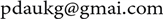 ; Mohammad Reza Faisal,
 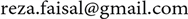 ; Bahriddin Abapihi,
  ; Bedy Purnama,
  ; Mera Kartika Delimayanti,
  ; Mamoru Kubo,
  ; Kenji Satou,
Keywords: Protein Phosphorylation, Phosphorylation Site Prediction, Sequence Feature, Feature Selection with Grid Search
Copyright © 2018 by authors and Scientific Research Publishing Inc.
This work is licensed under the Creative Commons Attribution International License (CC BY 4.0).
http://creativecommons.org/licenses/by/4.0/


Received: May 27, 2018 Accepted: June 26, 2018 Published: June 29, 2018; Copyright © 2018 by authors and Scientific Research Publishing Inc.; This work is licensed under the Creative Commons Attribution International License (CC BY 4.0).
ABSTRACT
Phosphorylation of protein is an important post-translational modification that enables activation of various enzymes and receptors included in signaling pathways. To reduce the cost of identifying phosphorylation site by laborious experiments, computational prediction of it has been actively studied. In this study, by adopting a new set of features and applying feature selection by Random Forest with grid search before training by Support Vector Machine, our method achieved better or comparable performance of phosphorylation site prediction for two different data sets.
1. Introduction
Phosphorylation is one of the most important post-translational modifications (PTMs) in eukaryotes. This occurs when a phosphate group is added to a protein by a kinase. The addition of phosphate group usually happens to Serine (S), Threonine, and Tyrosine (Y) [ 1 ]. It is also the common PTM, which occur in eukaryotic cell [ 2 ]. Between 30% and 50% proteins of eukaryotic cell undergo phosphorylation [ 3 ].
In the past, experimental approach such as mass spectrometry (MS/MS) [ 4 ] has been commonly used to identify phosphorylation sites. However, implementing this approach has several disadvantages. Conducting experiment to predict phosphorylation sites is considered expensive and requires intensive labor. In addition, it also requires adequate technique, skill, and specific equipment.
Instead, computational approach (in silico) is becoming more common because of new computer technology development. These days, computers can process large number of data in a short time. This makes prediction of phosphorylation sites using computational approach becoming more popular. Trost and Kusalik provided summarization of various technique approach, data, and tools that can be applied to predict phosphorylation site using computational approach [ 5 ].
In general, phosphorylation site prediction can be classified into two approaches: kinase-specific phosphorylation site prediction and non-kinase-specific (general) phosphorylation site prediction. Kinase-specific prediction approach requires both protein sequence and the type of kinase for phosphorylation to conduct prediction. The other approach is non-kinase-specific, which only requires protein sequence. Xue and Trost provided comparisons of these two approaches [ 5 , 6 ]. The main disadvantage of kinase-specific approach is that the publicly available information about the type of kinase is limited, especially for human kinase [ 7 ]. Therefore, non-kinase-specific approach is more popular to predict phosphorylation site [ 8 ].
There are various methods proposed for the prediction. For example, Blom used neural network (NN) approach to predict eukaryotic protein phosphorylation site based on sequence and structure of proteins [ 9 ]. Kim proposed a prediction method using support vector machine (SVM) [ 10 ].
In this paper, we propose a new prediction method for non-kinase-specific phosphorylation site. By adopting a new combination of a classifier, features, and feature selection algorithm, we improved the performance of prediction. We measured the result of feature selection and classification and compared it with existing methods. We also tested our method with an independent data set and analysis of the classification result.
2. Materials and Methods
2.1. Data Sets
In this work, we followed the preparation step done by Ismail [ 11 ]. The dataset we use were downloaded from the Phospho SVM website [ 12 ]. The phosphorylation site data set is P.ELM version 9 [ 13 ]. The data set contains phosphorylated sequences at the position of Serine (S), Threonine (T), and Tyrosine (Y). These sequences were also checked for redundancy and sequences that had similarity more than 30% were removed. Table 1 shows the number of sequences and number of sites for Serine, Threonine, and Tyrosine, respectively.
We generated fixed-length protein sequences using window size 9, which have phospholyratable residues (Serine, Threonine, or Tyrosine) at the center of them. If the center residue of the sequence is known as phosphorylated, the sequence is “positive”, otherwise “negative”. For positive and negative sequences, redundant ones were removed using skipredundant [ 14 ]. The parameters for redundancy removal are as follows: acceptable threshold percentage of similarity was set to 0% - 20%, value for gap opening penalty to 10, and gap extension penalty to 0.5. Table 2 shows the number of positive and negative sequences before and after removing redundant sequences for each residue.
The number of negative sequences after redundancy removal for Serine, Threonine, and Tyrosine residues are: 4771, 3343, and 898, respectively. We then randomly selected negative sequences for each residue with the same number of negative sequences in the work of Ismail.
Using the same window size and method, we also generated sequences from PPA data set downloaded from the Phospho SVM website for conducting performance evaluation by independent data set. PPA is a database for providing information of phosphorylation sites in Arabidopsis and a predictor for plant-specific phosphorylation site [ 15 ]. After removal of redundant sequences, we randomly selected positive and negative sequences based on the work of Ismail. Table 3 shows number of positive and negative phosphorylation sites for each amino acid. In order to make the data set well-balanced, the numbers of positive and negative sequences were set to equal.

Table 1. P.ELM data set of phosphorylation site from PhosphoSVM website.
Table 2. Number of sequences before and after removing redundant sequence for window size = 9.
Table 3. PPA data set as the independent data set.
2.2. Methods
2.2.1. Feature Extraction
Using the fixed-length sequences, we conducted feature extraction to represent them as vectors of numerical values. We used three different programs to extract features: PROFEAT (2016), PSI-BLAST, and protr.
PROFEAT (2016) is a web server for extracting features from protein sequences [ 16 ]. We used it to generate the following feaures: Amino Acid Composition, Dipeptide Composition, Normalized Moreau-Broto Autocorrelation Descriptor, Moran Autocorrelation Descriptor, Moran Autocorrelation Descriptor, Geary Autocorrelation Descriptor, Composition, Transition, Distribution Descriptor, Amphiphilic Pseudo-Amino Acid Composition, and Total Amino Acid Properties. For Position Specific Scoring Matrix (PSSM) features, we used PSI-BLAST [ 17 ]. In addition, an R package called protrwas used to produce the following features: BLOSUM and PAM Matrices for the 20 Amino Acid, Amino Acid Properties Based Scales Descriptor (Protein Fingerprint), Scales-based Descriptor derived by Principal Components Analysis, Scales-based Descriptor derived by Multidimensional Scaling, Conjoint Triad Descriptors, and Sequence-Order-Coupling Number [ 18 ]. Details of these features are described below. Except three features (CTD, SOCN, QSO), most of the features are not used in Ismail’s work.
• Amino Acid Composition (AAC)
Amino Acid Composition is defined as the fraction of each amino acid in a protein sequence [ 19 ]. For all 20 amino acids, the fraction is calculated using this equation.
(1)
where i is a spesific type of amino acid
• Dipeptide Composition (DPC)
Dipeptide Composition generates 400 fixed-length numeric information based on the input protein sequences. It encapsulates information about the fraction of amino acid as well as their local order. It is calculated using Equation (2):
(2)
where dep(i) is one dipeptide i of 400 dipeptides.
• Normalized Moreau-Broto Autocorrelation Descriptors (NMB)
Before we calculate Normalized Moreau-Broto Autocorrelation, we must define Moreau-Broto Autocorrelation. It can be define using Equation (3):
(3)
where Pi and Pi+d are the amino acid property at position i and i + d, respectively. Normalized Moreau-Broto Autocorrelation is defined using Equation (4) [ 20 ]:
(4)
where d = 1, 2, 3, ∙∙∙, 30.
When we usePROFEAT, the value of nlag should be lower than the size of the sequence. Since the window size is 9, we setnlag = 8.
• Moran Autocorrelation Descriptors (MORAN)
Moran Autocorrelation can be calculated using Equation (5):
(5)
where is the avarege of Pi. In the use of PROFEAT, we setnlag = 8.
• Geary Autocorrelation Descriptors (GEARY)
Geary Autocorrelation can be defined using Equation (6):
(6)
In the use of PROFEAT, we setnlag = 8.
• Composition, Transition, Distribution (CTD)
Composition, Transition, Distribution represent the amino acid distribution patterns of a certain structural or physicochemical property from a protein sequences. These features are calculated as follows: the protein sequence is transformed into a sequence of a specific physicochemical or structural properties of residue. Twenty amino acids are divided into three groups [ 20 , 21 ].
Composition (C), Transition (T), and Distribution (D) are then calculated for a given attribute to describe the global percent composition if the three groups of amino acids in a protein, the percent frequencies with which the attribute changes its index along the entire length of the protein, and the distribution pattern of attribute along the sequence, respectively.
• Sequence-Order-Coupling Number (SOCN)
Sequence-Order-Coupling Number can be used to represent amino acid distribution pattern of a specific physicochemical property along a protein sequence. The dth rank of sequence-order-coupling number can be calculated using Equation (7):
(7)
where di,i+d is the distance between two amino acid at position i and i + d. In the use of protr, we also setnlag = 8.
• Quasi-Sequence-Order Descriptors (QSO)
Quasi-Sequence-Order Descriptors can be calculated using Sequence-Order-Coupling Number. For each amino acid type, the type-1 Quasi-Sequence-Order Descriptors is calculated using Equation (8):
(8)
where fr is the normalized occurrence of amino acid type i and w is the weighting factor, w = 0.1. The type-2 Quasi-Sequence-Order Descriptors is calculated using Equation (9):
(9)
In the use of PROFEAT, we setnlag = 8.
• Amphiphilic Pseudo-Amino Acid Composition(APAAC)
Before we calculate Amphiphilic Pseudo-Amino Acid Composition, we must define Pseudo-Amino Acid Composition (PAAC) [ 22 ]. First, three variables are generated from the original hydrophobicity values , hydrophilicity values , and side chain masses of 20 amino acids (i = 1, 2, 3, ∙∙∙, 20).
(10)
(11)
(12)
Then, a correlation function can generated as:
(13)
From which, sequence order-correlated factors are defined as:
(14)
where λ is parameter. Let fi be the normalized frequency of 20 amino acids in the protein sequence, a set of 20 + λ descriptors called the PAAC can be defined using Equation (15):
(15)
where w = 0.05. From Equation (10) and Equation (11), the hydrophobicity and hydrophilicity correlation can be define as:
(16)
Then, sequence order factor can be define using Equation (17):
(17)
Finally, APAAC can be calculated using Equation (18):
(18)
In the use of PROFEAT, we set weight factor = 0.05 and lamda = 8.
• Total Amino Acid Properties (AAP)
Total Amino Acid Properties for a specific physicochemical property i is defined using Equation (19):
(19)
where represents the property i of amino acid Rj that is normalized between 0 and 1.N is the length of the protein sequence. is calculated using Equation (20):
(20)
where is the original amino acid property i for residue j. and are the minimum and the maximum values of the original amino acid property i, respectively.
• Position Specific Scoring Matrix (PSSM)
PSSM features were generated using PSI-BLAST against a local database generated from the phosphorylation data set.
• BLOSUM and PAM Matrices for the 20 Amino Acid (BLOSUM)
In the use of protr, we setk = 5, lag = 3, and Matrix type = AABLOSUM45.
• Amino Acid Properties Based Scales Descriptor (Protein Fingerprint) (ProtFP)
In the use of protr, we set pc = 5, lag = 5, index vector for Amino Acid Index = (160:165, 258:296).
• Scales-based Descriptor derived by Principal Components Analysis (SCALES)
In the use of protr, we set pc = 7, lag = 5, properties matrix = AA index (7:26).
• Scales-based Descriptor derived by Multidimensional Scaling (MDDSCALES)
In the use of protr, we set lag = 8.
• Conjoint Triad Descriptors (CTriad) [ 22 ]
2.2.2. Feature Selection
Random Forest was introduced by Breiman [ 23 ]. Random Forest method works as a collection of large number of decision trees randomly generated and not correlated to each other. This method is widelyapplied to classification problems.
In Random Forest, Gini impurity index (GII) is used to measure feature importance. GII represents how often randomly chosen element from the data set would be classified incorrectly if it was randomly classified based on the distribution of classes in the subset. We use Gini Index to rank important features that can be used for the classification algorithm.
In [ 11 ], Ismail also attempted the same feature selection and top 100 features were selected. In contrast, we conducted grid search to find the best set of selected features.
2.2.3. Classification
Vapnik [ 24 ] proposed support vector machine (SVM) as a classification method. It is a popular classifier widely applied to various problems including phosphorylation site prediction. SVM produces an optimal hyperplane separation between the classes. Here, optimal means finding the maximum margin around the separating hyperplane. In this work, we adopted Gaussian (also known as radial basis function) kernel for SVM.
2.2.4. Evaluation
10-fold cross-validation was repeated 10 times to measure the average performance of the P.ELM data. To measure the performance for the PPA data set, which is used for the independent data set, leave-one-out cross-validation (LOOCV) was conducted.
The metricsused to measure the classification performance are: Accuracy, Sensitivity, Specificity, F1 score, and Matthew’s Correlation Coefficient (MCC). These metrics are defined in the following equations:
(21)
(22)
(23)
(24)
(25)
where TP, TN, FP, and FN are the abbreviation for true positive, true negative, false positive, and false negative. In this work, Area under the ROC curve (AUC) is also measured.
3. Result and Discussion
3.1. P.ELM Data Set
3.1.1. Feature Selection
Gini impurity index (GII) in Random Forest was used to measure the importance of the features. For P.ELM data set, we conducted 10-fold cross validation repeated 10 times. For each fold in each iteration, we generate a list of important features based on the training data. Then we average the value GII of each features from the 100 list features we generated before. To give insight of which features that effects the classification, we listed the top twenty features for each residue in Figure 1. Composition, Transition, and

Figure 1. Top twenty importanct features for Serine (top), Threonine (middle), Tyrosine (bottom). The akronims of the group features are: Amino Acid Composition (AAC);Dipeptide Composition (DPC); Normalized Moreau-Broto Descriptors (NMB); Moran Autocorrelation Descriptors (MORAN); Geary Autocorrelation Descriptors (GEARY); Composition, Transition, Distribution (CTD); Quasi-Sequence-Order Descriptors (QSO); Amphiphilic Pseudo-Amino Acid Composition (APAAC); Total Amino Acid Properties (AAP); Position Specific Scoring Matrix (PSSM); BLOSUM and PAM Matrices the 20 Amino Acid (BLOSUM); Amino Acid Properties Based Scales Descriptors (ProtFP); Scale-based Descriptor derived by Principal Components Analysis (SCALES); Scale-based Descriptor derived by Multidimensional Scaling (MDSSCALES); Conjoint Triad Descriptor (Ctriad); 16: Sequence-Order-Coupling Number (SOCN). The number prefixed to a group name is just an identifier to descriminate different features in the same group.
Distribution (CTD) dominates the features for Serine (60% of all 20 features), and followed by Position Specific Scoring Matrix (PSSM) and Quasi-Sequence-Order (QSO), 15% and 10%, respectively. Although not as large as Serine, CTD still dominates the features for Threonine residue (35% of all 20 features). Furthermore, as the same as Serine, PSSM is the second dominate feature by 20%. In addition, the third dominant features is QSO by 10%. In contrast, for Tyrosine, MDSSCALES dominates the list by 30% from all 20 features, followed by CTD and QSO.
From Figure 1, we can assume that CTD group features plays an important role, to predict phosphorylation site for Serine and Threonine. However, for Tyrosine it is not a top important feature. It suggests the specialty of Tyrosine in protein phosphorylation in comparison with Serine and Threonine.
3.1.2. Classification Result
The performance of our proposed method is shown in Table 4. In general, we can see that there is an improvement if we implement feature selection before conducting class prediction. Without feature selection (i.e. using all the 2292 features), the prediction performances were quite low in all six metrics.
By implementing feature selection with grid search for finding the best set of features, performances were improved greatly. For instance, using only averagely top 271 important features, Serine increased its accuracy and having the highest accuracy 96.46%, followed by Threonine 92.22% by using averagely top 224 important features. For Tyrosine, by using averagely top 1635important features, achieved its best performance, which is 80.19%. Based on the comparison before using and after using feature selection, Threonine has the largest percentage of increase accuracy, which is 40.43%, followed by Serine 34.46%, and Tyrosine 24.65%.
Since feature selection decreased the performance in Ismail’s work, it is an important finding that under an appropriate combination of classifier and features, feature selection could improve the performance of protein phosphorylation site prediction.
In this work, we also compared the result of our method with existing methods for predicting phosphorylation site. The compared methods are as follows: Netphos [ 9 ], Netphos K [ 25 ], GPS 2.1 [ 26 ], Swaminathan, NetPhos [ 9 ], PPRED [ 8 ], Musite [ 27 ], Phospho SVM [ 12 ], and RF-Phos [ 11 ]. Table 5 shows the performance comparison between our method with other methods. For Serine and Threonine, our method achieved highest AUC, sensitivity, and MCC. However, specificity using Threonine data set is lower than the result of RF-Phos. On the other hand, our method using Tyrosine data set achieved a lower AUC, specificity, and MCC, in comparison with the result of RF-Phos. In addition, only sensitivity achieved the highest score.
Table 4. Performance of Classification using all of the features (2292 features) and best result of features selection.
Table 5. Comparsion of performance several methods to predict phosphorylation site for residue: Serine, Threonine, and Tyrosine.
3.2. PPA Data Set
Using the PPA data set as an independent data set, we also conducted feature selection by Random Forest and classification by SVM.
3.2.1. Feature Selection
We used the same features importance value as the P.ELM data set, that is Gini impurity index from Random Forest. Using PPA data set, we conducted leave-one-out cross validation. For each fold, we generate a list for important featured based on the training data. The number of feature list for each residue equals the number of samples in the data set. We measure the average GII value for each features from all list feature. The top twenty important features are shown in Figure 2. CTD dominates the top twenty features for Serine by 75% of all top twenty features, then followed by QSO only 10%. For Threonine, MDSSCALES dominates the top twenty features by 30%, second place CDT and QSO appear 20%. For Tyrosine, SCALES features dominates by 50%, followed by MDSSCALES by 20% of the top twenty features.
3.2.2. Classification Result
In general, as it is shown in Table 6, we can see that without feature selection, for all three data set, the accuracy is lower than 60%. However, there is an improvement if we implement feature selection before conducting class prediction. Threonine has the highest accuracy 91.18% using 772 features, then followed by Serine, using 1316 feature achieving 87.66% accuracy. Tyrosine, using 160 features, has the lowest accuracy in comparison with the other two data sets, achieving 57.84%.
If we compare the increase of performance between not using feature selection and feature selection, Threonine achieved63.18% increase of accuracy, followed by Serine 49.92% increase. Serine has the lowest increase of accuracy which is 59.65%.
We also compared our classification result with the ones in other researches. The method we comparedare: Netphos K, GPS 2.1, NetPhos, PHOSPHER, Musite, Phospho SVM, and RF-Phos. In Table 7, we can see that our method has a higher performance in sensitivity, specificity, and MCC for Serine and Threonine residue. For Tyrosine, our method could not outperform other results from previous work.

Figure 2. Top twenty importanct features for Serine (top), Threonine (middle), Tyrosine (bottom) using the independet data set.
Table 6. Performance of Classification using all of the features (2292 features) and best result of features selection using the independent data set.
Table 7. Comparsion of performance several methods to predict phosphorylation site using the independent data set for residue: Serine, Threonine, and Tyrosine.
4. ConclusionS
We proposed a non-kinase-specific method to predict phosphorylation site by applying feature selection and support vector machine. The features were generated from 16 groups of amino acid feature extraction methods. As it is shown from the top twenty important features for P.ELM and PPA data sets, the most important feature group was Composition, Transition, and Distribution (CTD) for Serine and Threonine residues. Using the P.ELM data set, our method achieved accuracy of 0.9646, 0.9222, and 0.8019 for Serine, Threonine, and Tyrosine, respectively. We also conducted classification for the PPA data set as an independent data set. Our method achieved 0.8766, 0.9118, and 0.5784 accuracy for Serine, Threonine, and Tyrosine residue, respectively.
In this study, we did not use most of features adopted in [ 11 ] except CTD, SOCN, and QSO. By incorporating such features to our method, we can expect further improvement of performance of predicting protein phosphorylation site from sequence.
Acknowledgements
In this research, the super-computing resource was provided by Human Genome Center, the Institute of Medical Science, the University of Tokyo. Additional computation time was provided by the super computer system in Research Organization of Information and Systems (ROIS), National Institute of Genetics (NIG). This work was supported by JSPS KAKENHI Grant Number 26330328.
Cite this paper
References
- 1. GenBank and WGS Statistics. https://www.ncbi.nlm.nih.gov/genbank/statistics/
- 2. UniProt Consortium (2014) UniProt: A Hub for Protein Information. Nucleic Acids Research, 43, D204-D212.
- 3. Xing, Z., Pei, J. and Keogh, E. (2010) A Brief Survey on Sequence Classification. ACM SIGKDD Explorations Newsletter, 12, 40-80. https://doi.org/10.1145/1882471.1882478
- 4. Borozan, I., Watt, S. and Ferretti, V. (2015) Integrating Alignment-Based and Alignment-Free Sequence Similarity Measures for Biological Sequence Classification. Bioinformatics, 31, 1396-1404. https://doi.org/10.1093/bioinformatics/btv006
- 5. Chen, L. and Guo, G. (2014) Nearest Neighbor Classification of Categorical Data by Attributes Weighting. Expert Systems with Applications, 42, 3142-3149. https://doi.org/10.1016/j.eswa.2014.12.002
- 6. Iqbal, M.J., Faye, I., Samir, B.B. and Said, A.M. (2014) Efficient Feature Selection and Classification of Protein Sequence Data in Bioinformatics. The Scientific World Journal, 2014, Article ID: 173869.
- 7. Weitschek, E., Cunial, F. and Felici, G. (2015) LAF: Logic Alignment Free and Its Application to Bacterial Genomes Classification. BioData Mining, 8, 2015. https://doi.org/10.1186/s13040-015-0073-1
- 8. Pham, T.H., Tran, T.B., Ho, T.B., Satou, K. and Valiente, G. (2005) Qualitatively Predicting Acetylation and Methylation Areas in DNA Sequences. Genome Informatics, 16, 3-11.
- 9. Pokholok, D.K., Harbison, C.T., Levine, S., Cole, M., Hannett, N.M., Lee, T.I., Bell, G.W., Walker, K., Rolfe, P.A., Herbolsheimer, E., Zeitlinger, J., Lewitter, F., Gifford, D.K. and Young, R.A. (2005) Genome-Wide Map of Nucleosome Acetylation and Methylation in Yeast. Cell, 122, 517-527. https://doi.org/10.1016/j.cell.2005.06.026
- 10. Higashihara, M., Rebolledo-Mendez, J.D., Yamada, Y. and Satou, K. (2008) Application of a Feature Selection Method to Nucleosome Data: Accuracy Improvement and Comparison with Other Methods. WSEAS Transactions on Biology and Biomedicine, 5, 153-162.
- 11. Li, J. and Wong, L. (2003) Using Rules to Analyse Bio-Medical Data: A Comparison between C4.5 and PCL. Proceedings of Advances in Web-Age Information Management 4th International Conference, Chengdu, 17-19 August, 254-265. https://doi.org/10.1007/978-3-540-45160-0_25
- 12. Nguyen, N.G., Tran, V.A., Ngo, D.L., Phan, D., Lumbanraja, F.R., Faisal, M.R., Abapihi, B., Kubo, M. and Satou, K. (2016) DNA Sequence Classification by Convolutional Neural Network. Journal of Biomedical Science and Engineering, 9, 280-286. https://doi.org/10.4236/jbise.2016.95021
- 13. Guo, S.H., Deng, E.Z., Xu, L.Q., Ding, H., Lin, H., Chen, W. and Chou, K.C. (2014) iNuc-PseKNC: A Sequence-Based Predictor for Predicting Nucleosome Positioning in Genomes with Pseudo k-Tuple Nucleotide Composition. Bioinformatics, 30, 1522-1529. https://doi.org/10.1093/bioinformatics/btu083
- 14. Tahir, M. and Hayat, M. (2016) iNuc-STNC: A Sequence-Based Predictor for Identification of Nucleosome Positioning in Genomes by Extending the Concept of SAAC and Chou’s PseAAC. Molecular BioSystems, 12, 2587- 2593. https://doi.org/10.1039/C6MB00221H
- 15. Awazu, A. (2016) Prediction of Nucleosome Positioning by the Incorporation of Frequencies and Distributions of Three Different Nucleotide Segment Lengths into a General Pseudo k-Tuple Nucleotide Composition. Bioinformatics, 33, 42-48. https://doi.org/10.1093/bioinformatics/btw562
- 16. Karatzoglou, A., Smola, A., Hornik, K. and Zeileis, A. (2004) Kernlab—An S4 Package for Kernel Methods in R. Journal of Statistical Software, 11, 1-20. https://doi.org/10.18637/jss.v011.i09
- 17. Liaw, A. and Wiener, M. (2002) Classification and Regression by Randomforest. R News, 2, 18-22. http://CRAN.R-project.org/doc/Rnews/
- 18. Chen, W., Feng, P., Ding, H., Lin, H. and Chou, K.C. (2015) Using Deformation Energy to Analyze Nucleosome Positioning in Genomes. Genomics, 107, 69-75. https://doi.org/10.1016/j.ygeno.2015.12.005
- 19. Yi, X.F., He, Z.S., Chou, K.C. and Kong, X.Y. (2012) Nucleosome Positioning Based on the Sequence Word Composition. Protein and Peptide Letters, 19, 79-90. https://doi.org/10.2174/092986612798472811
- 20. Hunter, T. (2000) Signaling—2000 and Beyond. Cell, 100, 113-127. https://doi.org/10.1016/S0092-8674(00)81688-8
- 21. Khoury, G.A., Baliban, R.C. and Floudasa, C.A. (2011) Proteome-Wide Post-Translational Modification Statistics: Frequency Analysis and Curation of the Swiss-Prot Database. Scientific Report, 1. https://doi.org/10.1038/srep00090
- 22. Pinna, L.A. and Ruzzene, M. (1996) How Do Protein Kinases Recognize Their Substrates? Biochimica et Biophysica Acta (BBA)—Molecular Cell Research, 1314, 191-225.
- 23. Newman, R.H., Zhang, J. and Zhu, H. (2014) Toward a Systems-Level View of Dynamic Phosphorylation Networks. Frontier in Genetics. https://doi.org/10.3389/fgene.2014.00263
- 24. Trost, B. and Kusalik, A. (2011) Computational Prediction of Eukaryotic Phosphorylation Sites. Bioinformatics, 27. https://doi.org/10.1093/bioinformatics/btr525
- 25. Xue, Y., Gao, X., Cao, J., Liu, Z., Jin, C., Wen, L., Yao, X. and Ren, J. (2010) A Summary of Computational Resources for Protein Phosphorylation. Current Protein and Peptide Science, 11, 485-496. https://doi.org/10.2174/138920310791824138
- 26. Newman, R.H., Hu, J., Rho, H.-S., Xie, Z., Woodard, C., Neiswinger, J., Ni, Q., et al. (2013) Construction of Human Activity—Based Phosphorylation Networks. Molecular Systems Biology, 9.
- 27. Biswas, A.K., Noman, N. and Sikder, A.R. (2010) Machine Learning Approach to Predict Protein Phosphorylation Sites by Incorporating Evolutionary Information. BMC Bioinformatcis, 11. https://doi.org/10.1186/1471-2105-11-273
- 28. Blom, N., Gammeltoft, S. and Brunak, S. (1999) Sequence and Structure-Based Prediction of Eukaryotic Protein Phosphorylation Sites. Journal of Molecular Biology, 294, 1351-1362. https://doi.org/10.1006/jmbi.1999.3310
- 29. Kim, J.H., Lee, J., Oh, B., Kimm, K. and Koh, I. (2004) Prediction of Phosphorylation Sites Using SVMs. Bioinformatics, 3179-3184. https://doi.org/10.1093/bioinformatics/bth382
- 30. Ismail, H.D., Jones, A., Kim, J.H., Newman, J.H. and KC, D.B. (2016) RF-Phos: A Novel General Phosphorylation Site Prediction Tool Based on Random Forest. BioMed Research International, 12. https://doi.org/10.1155/2016/3281590
- 31. Dou, Y., Yao, Y. and Zhang, Y. (2014) PhosphoSVM: Prediction of Phosphorylation Sites by Integrating Various Protein Sequence Attributes with a Support Vector Machine. Amino Acids, 46, 1459-1469. https://doi.org/10.1007/s00726-014-1711-5
- 32. Dinkel, H., Chica, C., Via, C., Gould, C.M., Jensen, L.J., Gibson, T.J. and Diella, F. (2011) Phospho.ELM: A Database of Phosphorylation Sites—Update 2011. Nucleic Acids Research, 39, D261-D267. https://doi.org/10.1093/nar/gkq1104
- 33. Sikic, K. and Carugo, O. (2010) Protein Sequence Redundancy Re-duction: Comparison of Various Methods. Bioinformation, 5, 234-239. https://doi.org/10.6026/97320630005234
- 34. Heazlewood, J.L., Durek, P., Hummel, J., Selbig, J., Weckwerth, W., Walther, D. and Schulze, W.X. (2007) PhosPhAt: A Database of Phosphorylation Sites in Arabidopsis thaliana and a Plant-Specific Phosphorylation Site Predictor. Nucleic Acids Research, 36, D1015-D1021. https://doi.org/10.1093/nar/gkm812
- 35. Rao, H.B., Zhu, F., Yang, G.B., Li, R. and Chen, Z. (2011) Update of PROFEAT: A Web Server for Computing Structural and Physicochemical Features of Proteins and Peptides from Amino Acid Sequence. Nucleic Acids Research, 39, W385-W390. https://doi.org/10.1093/nar/gkr284
- 36. Bergman, N.H. (2007) Comparative Genomics: Volumes 1 and 2. Humana Press, Totowa. https://doi.org/10.1007/978-1-59745-515-2
- 37. Xiao, N., Cao, D.-S., Zhu, M.-F. and Xu, Q.-S. (2015) Protr/ProtrWeb: R Package and Web Server for Generating Various Numerical Representation Schemes of Protein Sequences. Bioinformatics, 31, 1857-1859. https://doi.org/10.1093/bioinformatics/btv042
- 38. Bhasin, M. and Raghava, G.P. (2004) Classification of Nuclear Receptors Based on Amino Acid Composition and Dipeptide Composition. Journal of Biological Chemistry, 279, 23262-23266. https://doi.org/10.1074/jbc.M401932200
- 39. Li, Z.R., Lin, H.H., Han, L.Y., Jiang, L., Chen, X. and Chen, Y.Z. (2006) PROFEAT: A Web Server for Computing Structural and Physicochemical Features of Proteins and Peptides from Amino Acid Sequence. Nucleic Acids Research, 34, W32-W37. https://doi.org/10.1093/nar/gkl305
- 40. Dubchak, I., Muchnik, I., Mayor, C., Dralyuk, I. and Kim, S.-H. (1999) Recognition of a Protein Fold in the Context of the SCOP Classification. Proteins: Structure, Function, and Bioinformatics, 35, 401-407. https://doi.org/10.1002/(SICI)1097-0134(19990601)35:4<401::AID-PROT3>3.0.CO;2-K
- 41. Shen, J., Zhang, J., Luo, X., Zhu, W., Yu, K., Chen, K., Li, Y. and Jiang, H. (2007) Predicting Protein-Protein Interactions Based Only on Sequences Information. Proceedings of the National Academy of Sciences, 104, 4337-4341. https://doi.org/10.1073/pnas.0607879104
- 42. Breiman, L. (2001) Random Forests. Machine Learning, 45, 5-32. https://doi.org/10.1023/A:1010933404324
- 43. Vapnik, V.N. (1998) Statistical Learning Theory. Wiley, New York.
- 44. Blom, N., Sicheritz-Pontén, T., Gupta, R., Gammeltoft, S. and Brunak, S. (2004) Prediction of Post-Translational Glycosylation and Phosphorylation of Proteins from the Amino Acid Sequence. Proteomics, 4, 1633-1649. https://doi.org/10.1002/pmic.200300771
- 45. Xue, Y., Liu, Z., Cao, J., Ma, Q., Gao, X., Wang, Q., Ren, J., et al. (2011) GPS 2.1: Enhanced Prediction of Kinase-Specific Phosphorylation Sites with an Algorithm of Motif Length Selection. Protein Engineering Design & Selection, 24, 255-260. https://doi.org/10.1093/protein/gzq094
- 46. Gao, J., Thelen, J.J., Dunker, A.K. and Xu, D. (2010) Musite, a Tool for Global Prediction of General and Kinase-Specific Phosphorylation Sites. Molecular & Cellular Proteomics, 9, 2586-2600. https://doi.org/10.1074/mcp.M110.001388