Journal of Biomedical Science and Engineering
Vol.6 No.3A(2013), Article ID:29493,10 pages DOI:10.4236/jbise.2013.63A042
Automated measurement of three-dimensional cerebral cortical thickness in Alzheimer’s patients using localized gradient vector trajectory in fuzzy membership maps
![]()
1Division of Radiology, Department of Medical Technology, Kyushu University Hospital, Fukuoka, Japan
2Department of Health Sciences, Faculty of Medical Sciences, Kyushu University, Fukuoka, Japan
3Department of Clinical Radiology, Graduate School of Medical Sciences, Kyushu University, Fukuoka, Japan
4Department of Neuropsychiatry, Graduate School of Medical Sciences, Kyushu University, Fukuoka, Japan
5Department of Health Sciences, Graduate School of Medical Sciences, Kyushu University, Fukuoka, Japan
Email: arimurah@med.kyushu-u.ac.jp
Received 14 January 2013; revised 22 February 2013; accepted 28 February 2013
Keywords: Alzheimer’s Disease (AD); Fuzzy C-Means Clustering (FCM); Three-Dimensional Cerebral Cortical Thickness; Localized Gradient Vector
ABSTRACT
Our purpose in this study was to develop an automated method for measuring three-dimensional (3D) cerebral cortical thicknesses in patients with Alzheimer’s disease (AD) using magnetic resonance (MR) images. Our proposed method consists of mainly three steps. First, a brain parenchymal region was segmented based on brain model matching. Second, a 3D fuzzy membership map for a cerebral cortical region was created by applying a fuzzy c-means (FCM) clustering algorithm to T1-weighted MR images. Third, cerebral cortical thickness was threedimensionally measured on each cortical surface voxel by using a localized gradient vector trajectory in a fuzzy membership map. Spherical models with 3 mm artificial cortical regions, which were produced using three noise levels of 2%, 5%, and 10%, were employed to evaluate the proposed method. We also applied the proposed method to T1-weighted images obtained from 20 cases, i.e., 10 clinically diagnosed AD cases and 10 clinically normal (CN) subjects. The thicknesses of the 3 mm artificial cortical regions for spherical models with noise levels of 2%, 5%, and 10% were measured by the proposed method as 2.953 ± 0.342, 2.953 ± 0.342 and 2.952 ± 0.343 mm, respectively. Thus the mean thicknesses for the entire cerebral lobar region were 3.1 ± 0.4 mm for AD patients and 3.3 ± 0.4 mm for CN subjects, respectively (p < 0.05). The proposed method could be feasible for measuring the 3D cerebral cortical thickness on individual cortical surface voxels as an atrophy feature in AD.
1. INTRODUCTION
Alzheimer’s disease (AD) is a major health and social problem in advanced countries with long life expectancy, such as Japan and the United States of America. According to recent estimates, as many as 2.4 million to 4.5 million Americans and 1.8 million Japanese have AD [1, 2]. AD is associated with atrophy of gray matter in the cerebral cortex, which leads to morphological changes, i.e., a decrease in the thickness of the cerebral cortex or an increase in the volume of cerebrospinal fluid (CSF) in the cerebral sulci and lateral ventricles (LVs), which can be measured in magnetic resonance (MR) images. Furthermore, the atrophy of gray matter occurring in early stages of AD is localized to specific regions such as the hippocampus, amygdala, entorhinal area, and medialtemporal cortex [3,4]. Querbes et al. [5] reported that patients with AD in early stages can be diagnosed using a normalized thickness index-based criterion. Because palliative medicines can delay the progression of AD, early diagnosis and treatment are highly important [6,7]. Therefore, neuroradiologists attempt to subjectively estimate the degree of atrophy by analyzing atrophic morphological changes on MR images such as the cerebral cortical thickness, but a diagnosis based on such analysis is not quantitative or reproducible.
Several methods have been developed for quantitative measurement of cerebral cortical thickness between the white matter and cortical surfaces based on the analysis coupled surfaces propagation using the level set method [8], Laplace’s equation from mathematical physics [9], the average least distance [10], the distance between linked vertices [11], and normal vectors derived using the level set method [12].
In the method of Jones et al. [9], the cortical thicknesses were measured by means of gradient vector trajectries in a virtual electromagnetic field, which was constructed to be analogous to the neuronal sublayers between the cortical surface and white matter surface. Their method, in which the gradient vectors were orthogonal to the nested sublayers, is considered to be reliable. Acosta et al. [13] developed a voxel-based method that is both accurate and computationally efficient by extending Jones’s method to a Lagrangian-Eulerian approach. A hollow sphere with an inner radius of 20 mm and external radius of 23 mm has a cortical thickness of 3 mm similar to the cerebral cortex, was constructed to evaluate their method. Their results showed that the cortical thickness was 3.04 ± 0.02 mm with a voxel size of 1 mm, which seems to be accurate and reliable. Therefore, in this study we adopted Jones’s basic idea for the measurement of the cortical thickness, which is to use the trajectory of the gradient vector in some 3D space, but we used a different method for calculating the gradient vectors.
Previous methods for measuring cortical thickness depended on the accuracy of determination of the boundary between the cerebral cortex and white matter regions. However, it can be very difficult to determine the boundary in the case of diffuse neuronal cell death, since the edges of white matter regions may be blurred or voxels of the cortex and white matter in the boundary may be mixed, making them appear fuzzy. In addition, past studies have not considered the voxel value information in MR images, which could include the atrophy information in the cerebral cortex. To overcome these issues, we employed fuzzy c-means (FCM) clustering [14-17]. We assumed that the 3D membership map in the FCM clustering can express the fuzzy boundary between the cerebral cortex and white matter regions, and the fuzzy framework can incorporate voxel value information related to the AD atrophy.
Our purpose in this study was to develop an automated method for measuring the 3D cerebral cortical thicknesses in AD patients based on 3D fuzzy membership maps derived from T1-weighted images, which includes atrophy information in the cerebral cortical regions. In the proposed method, the boundary between the cortical and white matter regions is determined on each cortical surface voxel by using membership profiles on trajectories of local gradient vectors in a fuzzy membership map, so that the white matter regions do not have to be segmented.
2. MATERIALS AND METHODS
2.1. Overall Algorithm
Figure 1 shows the overall scheme for measurement of the 3D cerebral cortical thickness. The proposed method consisted of mainly three steps as follows.
1) Segmentation of the brain parenchymal region based on a brain model matching.
2) Creation of a fuzzy membership map for the cerebral cortical region based on the FCM clustering algorithm [14-17].
3) Calculation of the cerebral cortical thickness using localized gradient vector trajectories in fuzzy membership maps.
2.2. Segmentation of the Brain Parenchymal Region
2.2.1. Initial Brain Parenchymal Region Based on Histogram Analysis
The background (BG) and CSF regions were removed from an original T1-weighted image based on a histogram analysis. Figure 2 shows a histogram of the original T1-weighted image. The histogram of the T1- weighted image could be divided into four portions that included three peaks, which correspond to the BG (the largest peak), CSF (the second largest peak), and the brain parenchyma and fat regions (the third largest peak), respectively. The two threshold values, TBG and TCSF, for reducing the BG and CSF regions, respectively, are shown in Figure 2. The inset figure shows the enlarged histogram without the background peak. The threshold value, TBG, for the background region was determined as TBG = MBG + kBGSDBG, where MBG and SDBG are the mean value and the standard deviation (SD), respectively. The values MBG and SDBG were determined from the first largest peak with more than a certain number of pixels, which was empirically set as 300,000 pixels in this study, and kBG is the constant, which was empirically set as 1.0. Similarly, the threshold value for reducing the CSF region, TCSF, was determined as TCSF = MCSF + kCSFSDCSF,
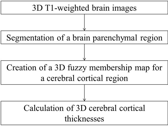
Figure 1. Overall scheme for the calculation of three-dimensional cortical thicknesses.
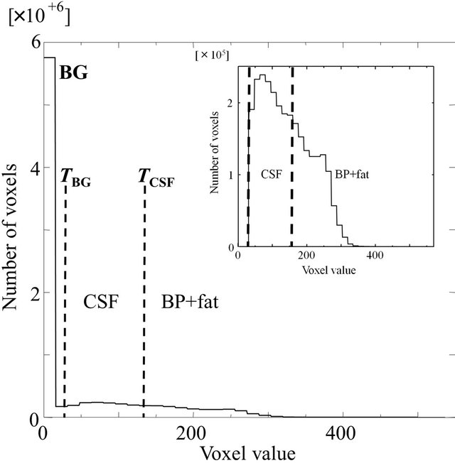
Figure 2. A histogram of an original T1- weighted image, where TBG and TCSF are the threshold values for reducing the background (BG) and CSF regions, respectively. The inset figure shows the enlarged histogram without the BG peak.
where MCSF and SDCSF are the mean value and the standard deviation, respectively, and kCSF is the constant, which was empirically set at –0.25. After reducing the CSF region, the initial brain parenchymal region was segmented by applying morphological processing and extracting the largest region.
2.2.2. Segmentation of the Brain Parenchymal Region with Brain Model Matching
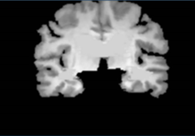
Figure 3 shows a flowchart for the segmentation of the brain parenchymal region using a brain model matching. The brain parenchymal model image shown in Figure 4(a) was manually created from a T1-weighted image of a cognitively normal (CN) subject, whose brain seemed to be of average size and shape (female, 71 years old; mini-mental state examination (MMSE) score: 30). A voxel value similar to those in the white matter regions was assigned to holes of the CSF regions in the LVs to avoid removing some portions of the brain parenchyma by the holes of lateral ventricles due to misregistration. The brain parenchymal region was segmented by registering and masking of the brain model image to each head region, in which the BG and CSF regions were removed, based on a global linear registration of an affine transformation [18,19] and a local non-linear registration of the free-form deformation (FFD) [20-23]. Figure 4 shows images of the segmentation of a brain parenchymal region: (a) an original brain model image; (b) a brain model image after global registration to a normalized image; (c) an image after local registration; (d) a brain parenchymal mask image; (e) a head region after removing CSF regions; and (f) a brain parenchymal region extracted from the head region (e) by the brain mask image (d).
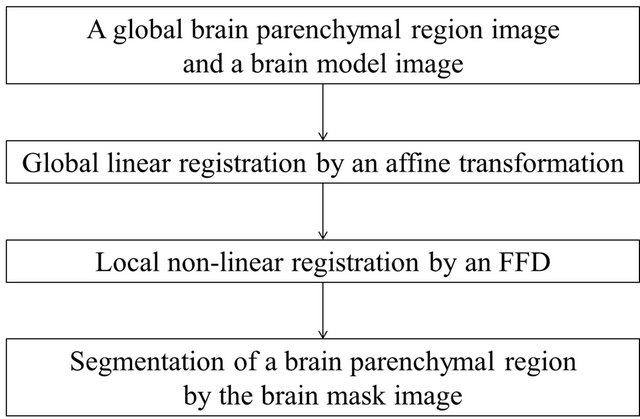
Figure 3. Flowchart for segmentation of the brain parenchymal regions based on a brain model matching.
 (a)
(a)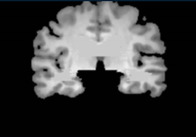 (b)
(b)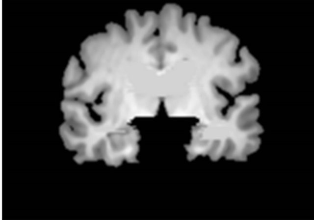 (c)
(c)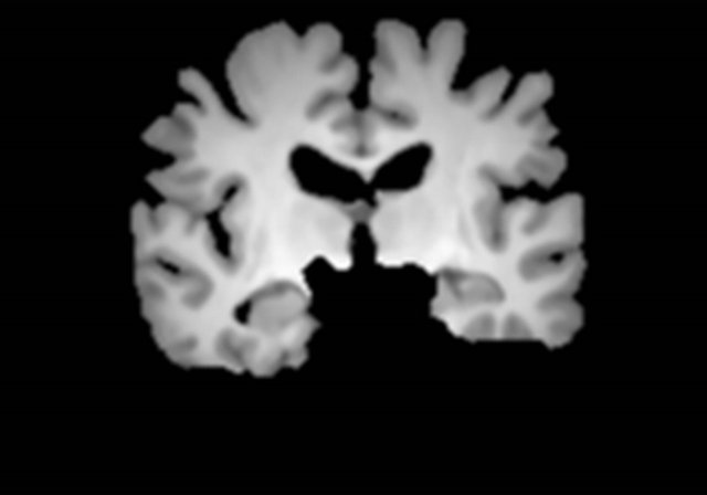 (d)
(d)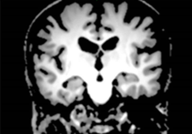 (e)
(e) (f)
(f)
Figure 4. Sample images of the segmentation of a brain parenchymal region: (a) An original brain model image; (b) A brain model image after global registration to a normalized image; (c) A brain model image after local registration; (d) A brain parenchymal mask image; (e) A head region after removing CSF regions; and (f) A brain parenchymal region extracted from the head region (e) by the brain mask image (d).
2.3. Creation of a Fuzzy Membership Map for the Brain Parenchymal Region Based on a Fuzzy C-Means Clustering
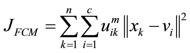
The 3D cerebral cortical thicknesses were measured in a fuzzy membership map space for the brain parenchymal region based on the FCM clustering, because the fuzzy membership can represent the phenomenon in which the cerebral cortical voxel value (gray color in T1-weighted image) gradually increases from the cortical surface to the white matter surface due to AD. The FCM clustering method assigns a class membership value to each voxel, depending on the similarity of the pixel to a particular class relative to all other classes [14-17]. In this study, all voxels were assigned two class membership values, i.e., cerebral cortical regions and white matter regions. The FCM method is performed by minimizing the following objective function with respect to the membership function uik and the centroids vi:
 (1)
(1)
where xk is the voxel value at a voxel k, c is the number of clusters, and n is the number of voxels. The membership functions are constrained to be positive and to satisfy the following equation:
 (2)
(2)
Here, the objective function is minimized when high membership values are obtained in areas where the objective voxel values are close to the centroid of one of the clusters, and low membership values are obtained where the objective voxel values are distant from the centroids. The parameter m is a weighting exponent that satisfies m > 1 and controls the degree of fuzziness. As m approaches 1, the membership functions become more crisp. On the other hand, as m increases, the membership functions become increasingly fuzzy. A region can be segmented by a certain threshold value for the membership value.
2.4. Measurement of the Cerebral Cortical Thickness Based on a Membership Profile
As mentioned in the Introduction section, we adopted the basic idea of Jones et al. [9], in which the cerebral cortical thicknesses were measured by the trajectories of gradient vectors in a virtual electromagnetic field that was constructed to be analogous to the neuronal sublayers between the cerebral cortical surface and white matter surface. In this study, we employed a fuzzy membership map of the brain parenchyma obtained from the T1- weighted image instead of the virtual electromagnetic field. Furthermore, the local gradient vector was calculated by the first-order polynomial within a 3D volume of interest (VOI) for reducing the impact of image noise on the local gradient. The local gradient vectors were almost orthogonal to the isosurface in the fuzzy membership map.
The 3D cerebral cortical thickness was measured based on a membership profile using a local gradient vector trajectory in a fuzzy membership map. First, a local gradient vector was calculated based on the firstorder polynomial within a VOI, but this local gradient vector was expected to proceed toward the white matter. The global gradient vector was obtained prior to calculation of the local gradient vector, whose direction should be within a 2π solid angle with respect to the global gradient vector. We assume that the gradient vector obtained from the VOI would have the potential to be robust against image noise, compared with the finite difference approximation for the first-order derivative. Second, a membership profile was constructed according to the trajectory of the local gradient vector from the cortical surface to the fully white matter regions. Finally, a 3D cerebral cortical thickness based on the membership profile was calculated on the local gradient trajectory.
2.4.1. Calculation of Local Gradient Vector Gl
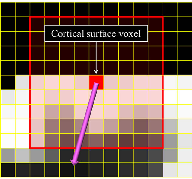
The local gradient vectors were derived from the firstorder polynomial in the VOI of the fuzzy membership map. Prior to calculation of the local gradient vector, the global gradient vector was obtained so that the local gradient vector direction would be within a 2π solid angle with respect to the global gradient vector. Figure 5 shows illustrations for calculation of global and local gradient vectors.
For calculation of the global gradient vector, a 9 × 9 × 9 VOI was set at the center of a surface voxel in a brain parenchymal region as shown in Figure 5(a). A firstorder polynomial was calculated in the VOI by using the following equation:
 (3)
(3)
Here, f(x, y, z) is the approximated membership value at (x, y, z) in a VOI, and a, b, c and d are constants. The vector (x, y, z) consisting of coefficients in Eq.3 is almost orthogonal to the isosurface of the fuzzy membership map. Therefore, the 3D gradient vector Gg from the surface of a cerebral cortical region to a white matter region is expressed by
 (4)
(4)
which is normalized to
 (5)
(5)
A local gradient vector was calculated in a 5 × 5 × 5 VOI, which was set at the center of an objective voxel as shown in Figure 5(b), by applying a first-order polynomial for this VOI in the same way as for the global gradient vector. Although the local gradient vector should proceed toward the white matter, the local gradient vectors may proceed in directions away from the white matter due to image noise. The global gradient vector was obtained prior to calculation of the local gradient vector, whose direction should be within a 2π solid angle with respect to the global gradient vector. Therefore, the local gradient vector was determined by using Eq.7 to calculate an angle θ between the global and local gradient vectors such that the local gradient vector direction would be within a 2π solid angle with respect to the global gradient vector. The angle θ between the global gradient vector Gg = (a b c)T and the local gradient vector Gl = (i j k)T was calculated by the following equation:
 (a)
(a)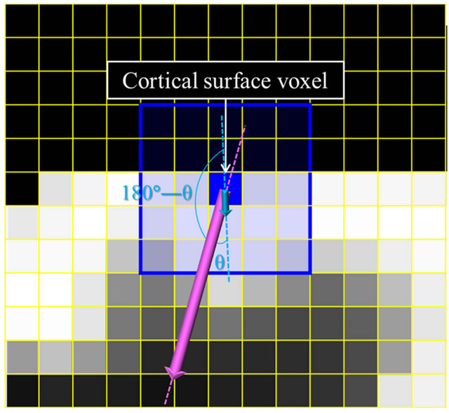 (b)
(b)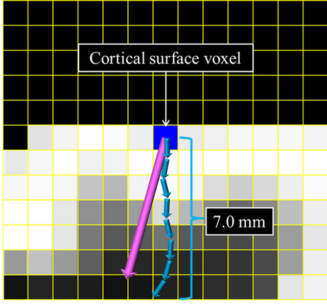 (c)
(c)
Figure 5. Illustrations for calculation of global and local gradient vectors: (a) A global gradient vector within a 9 × 9 × 9 volume-of-interest (VOI); (b) A local gradient vector within a 5 × 5 × 5 VOI; and (c) A trajectory of local gradient vectors.
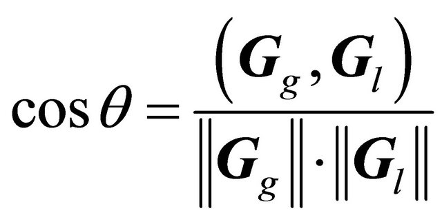 (6)
(6)
Consequently, the local gradient vector was obtained in one of the following two ways depending on the angle between the global and local gradient vectors:
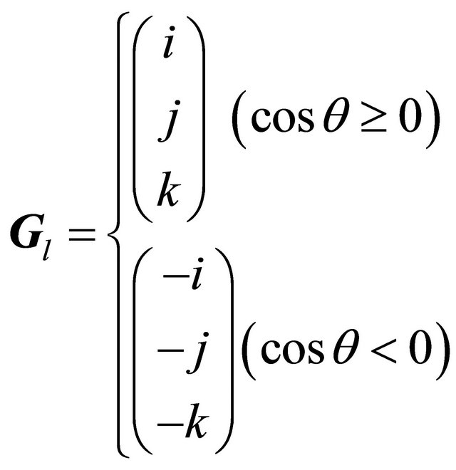 (7)
(7)
2.4.2. Measurement of the 3D Cerebral Cortical Thickness
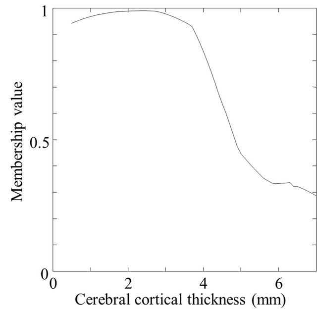
The 3D cerebral cortical thicknesses were measured by using membership profiles on trajectories of local gradient vectors in a fuzzy membership map. A trajectory of the local gradient vector was tracked until the sum of 0.1-mm-long local gradient vectors was 7.0 mm, as shown in Figure 5(c). A membership profile was constructed as a trajectory of the local gradient vector by connecting the membership value at each terminal point of the local gradient vector from the cortical surface to the fully white matter regions. The membership value at the terminal point of 0.1-mm-long local gradient vectors was calculated by using a linear interpolation method. The membership profile was normalized by setting the membership value at the cortical surface voxel and the minimum value of the profile as 1.0 and 0.0, respectively. Figure 6 shows a fuzzy membership profile on the trajectory of a local gradient vector from a white matter region to a cerebral cortical region. Finally, the 3D cerebral cortical thickness at each cortical surface voxel was estimated at a normalized membership value of 0.75 as the boundary between the cerebral cortical and white matter regions. The membership value of 0.75 was empirically determined so that the cerebral cortex could be segmented as accurately as possible for a spherical model with a cortical thickness of 3 mm. This spherical model will be described in a later section.
2.4.3. Segmentation of Ten Lobar Regions
In order to investigate the regional atrophy at the lobe level, the cerebral cortical thicknesses were separately evaluated in ten lobar regions. For this purpose, ten lobar regions were segmented by registering the lobar model image to each brain parenchymal image by using the affine transform and the FFD. The lobar model image was selected from a probabilistic reference system for the human brain at the International Consortium for Brain Mapping (ICBM) website of the Laboratory of Neuro Imaging (LONI) [24].
2.5. Spherical Brain Models for the Validation Test
Spherical brain models of known cortical thicknesses were used to evaluate the proposed method. The spherical
 (a)
(a)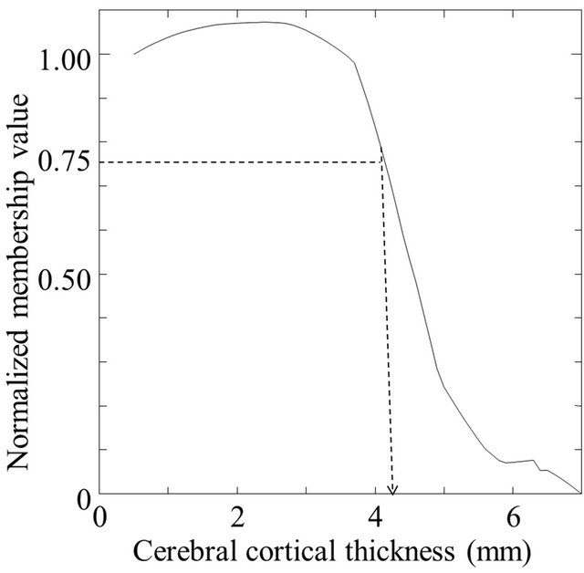 (b)
(b)
Figure 6. A fuzzy membership profile on a trajectory of a local gradient vector: (a) An original profile and (b) A profile normalized by the first value on the cortical surface.
brain models were of various noise levels and isotropic voxel sizes (resolutions), so that the ability of the proposed method to accurately determine cortical thicknesses under a variety of conditions could be analyzed.
A sphere of a brain model with an inner and outer radii of 37 mm and 40 mm, respectively, in which the cortical thickness was 3 mm, was generated in a fine grid space (1100 × 1100 × 1100) with an isotropic voxel size of 0.1 mm3. The pixel value spatial distribution of the cortical region in the inward direction to the center of the models was modeled by using the following error function:
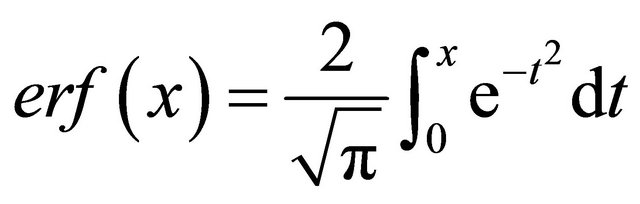 (8)
(8)
where x is the position in the inward direction. This function increases with the inward direction. Furthermore, brain models with three noise levels were produced by adding Gaussian random noise to the brain models so that the percentage of standard deviation of Gaussian noise to the mean voxel value in the whole original image was 2%, 5%, and 10%. The Gaussian noise was generated by converting uniform random numbers with a Box-Muller transform. To evaluate the robustness of the method to the noise, we prepared spherical brain models with three noise levels of 2%, 5%, and 10%. Figure 7 shows the spherical brain models with three noise levels of 2%, 5%, and 10% used for measurement of the cerebral cortical thicknesses, where the true thickness was 3 mm.
In addition to the three noise level models, we made two resolution models with voxel sizes of 0.5 mm and 1.0 mm by averaging a certain cubic VOI in order to investigate the impact of the partial volume effect on the proposed method.
2.6. Subjects and MRI Data
This study was approved by an institutional review board of our university. High-resolution T1-weighted images of whole brains acquired from 10 clinically diagnosed AD cases (age range: 63 - 84 years; median: 78.0 years) and 10 CN (67 - 86 years; 74.5 years) were randomly selected from among outpatients who visited our memory clinic from 2007 to 2008. Seven healthy volunteers were recruited, taking into account age matching with the AD patients, and they gave informed consent to undergo MR examination and for use of the data for research purposes. There was no statistical significant difference (p = 0.35) between the AD and CN groups in terms of age. The MMSE scores for AD patients and CN subjects ranged over 11 - 23 (median: 21) and 27 - 30 (median: 29), respectively. The 10 AD cases were determined by neuropsychiatrists based on the diagnostic and statistical manual of mental disorders (DSM)-IV criteria for the diagnosis of dementia of the Alzheimer’s type. These data were obtained with a 3.0-T MRI scanner (Intera Achieva 3.0 T Quasar Dual R2.1; Philips Electronics, Best, Netherlands) at our university hospital by using T1-weighted
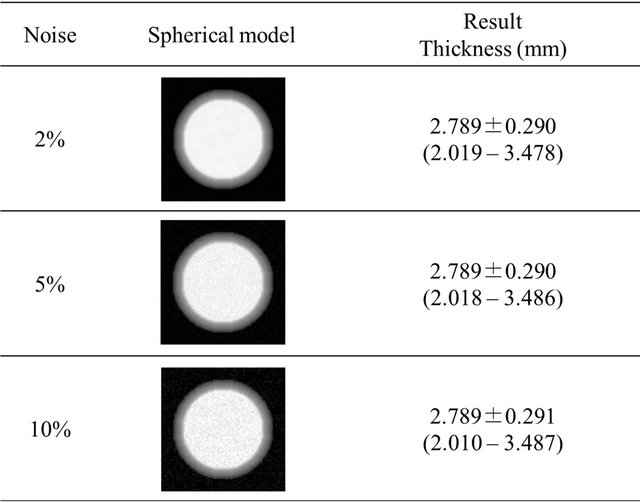
Figure 7. Spherical brain models with a cortical thickness of 3 mm used for the evaluation of cerebral cortical thicknesses.
3D turbo field echo (TFE) sequences (time of repetition (TR): 8.3 ms; time of echo (TE): 3.8 ms; time of inversion (TI): 240 ms; flip angle: 8 degrees; sensitivity encoding (SENSE) factor: 2; number of samples averaged (NSA): 1; field of view (FOV): 240 mm × 240 mm). The images were obtained in sagittal planes, and were reconstructed into 150 consecutive transverse slice images with a 1-mm-slice thickness and a matrix size of 240 × 240 pixels. All images were normalized from 0 to 1023 for voxel value, and preprocessed by a median filter for reduction of noise.
3. RESULTS
3.1. Validation Test for Spherical Brain Models
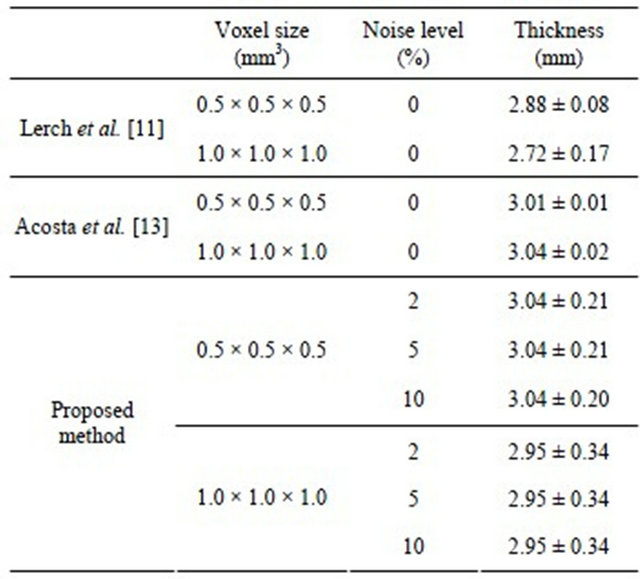
The cortical thicknesses with a voxel size of 0.5 × 0.5 × 0.5 mm3 for spherical brain models with three noise levels of 2%, 5%, and 10% were 3.041 ± 0.212, 3.041 ± 0.210, and 3.040 ± 0.204 mm, respectively. Cortical thicknesses with a voxel size of 1.0 × 1.0 × 1.0 mm3 for the three noise levels were 2.953 ± 0.342, 2.953 ± 0.342, and 2.952 ± 0.343 mm, respectively.
3.2. Clinical Magnetic Resonance Images
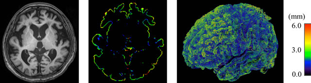
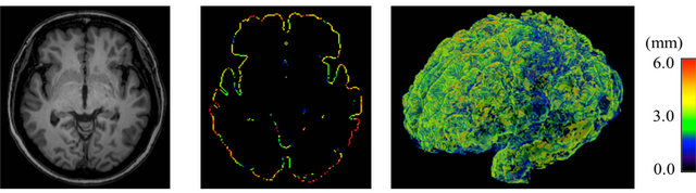
Table 1 shows the means of cerebral cortical thickness in ten lobar regions. The average cortical thicknesses in the right and left temporal lobes, and the left insula in AD cases were 3.32 ± 0.21, 3.16 ± 0.26, and 2.66 ± 0.23 mm, respectively. The cortical thicknesses for AD cases were significantly thinner than those in the corresponding regions in CN subjects, whose cortical thicknesses were 3.64 ± 0.40, 3.47 ± 0.32 and 3.00 ± 0.41 mm, respectively (p < 0.05). Figures 8 and 9 show color-coded maps of cerebral cortical thickness for an AD case and a CN subject produced by the proposed method. The AD case (Figure 8) appears to have a thinner cerebral cortex in the temporal or frontal lobes, compared with the CN subject (Figure 9).
4. DISCUSSION
Table 2 shows the comparison of results obtained by the three methods for measurement of cortical thickness in a spherical model with a 3 mm artificial cortical region. Our results seem to be close to the two past studies [11, 13], in spite of the changing levels of noise and resolution. Thus the proposed method may be robust against noise. As for the resolution, although we added some noise to the spherical model, our results were a little bit worse than those of Acosta et al. [13], who included no noise in their experiments.
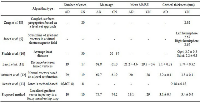
Table 3 shows a comparison of the results obtained by the 7 methods for measurement of cerebral cortical thickness in clinical cases. Zeng et al. [8] developed a method for the segmentation of cerebral cortical regions using coupled-surfaces propagation based on a level set approach, and for measurement of the cortical thickness.
Table 1. Means of cerebral cortical thickness in ten lobar regions.
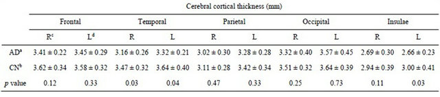
aAlzheimer’s disease patients; bClinically normal subjects; cRight hemisphere; dLeft hemisphere.
 (a) (b) (c)
Figure 8. Color-coded maps of cerebral cortical thickness in a patient with Alzheimer’s disease (age: 76 years; gender: female; mini-mental statement examination score: 21): (a) An original T1-weighted image; (b) A color-coded axial map; and (c) A color-coded volume-rendering map.
 (a) (b) (c)
Figure 9. Color-coded maps of cerebral cortical thickness in a patient with Alzheimer’s disease (age: 76 years; gender: female; mini-mental statement examination score: 21): (a) An original T1-weighted image; (b) A color-coded axial map; and (c) A color-coded volume-rendering map.
Table 2. Comparison of results obtained by three methods for the measurement of cortical thickness in a spherical model with a 3 mm artificial cortical region.
The mean cortical thickness for the 20 CN subjects was 2.92 mm. Jones et al. [9] presented a computerized method for measurement of the cortical thickness based on trajectories of gradient vectors in a virtual electromagnetic field. They found that the cortical thicknesses for the left and right hemispheres were 2.67 mm and 2.69 mm, respectively.
Fischls et al. [10] developed a method for thickness measurement of the cerebral cortex based on the average least distance, and reported that the average cortical thicknesses for 30 CN cases (20 - 37 years) were 2.7 ± 0.3 mm for gyri and 2.2 ± 0.3 mm for sulci. Lerch et al. [11] developed a method for cortical thickness measurement as the distance between vertices of the white matter and gray matter surfaces, which were fitted using deformable models, resulting in two surfaces with a huge number of polygons each. According to their results, the average cortical thickness was 3.1 ± 0.28 mm for 19 AD patients (mean age: 68.8; mean MMSE: 21.2 ± 4.6) and 3.74 ± 0.32 mm for 17 CN subjects (mean age: 61.0; mean MMSE: 29.3 ± 0.6). Arimura et al. [12] proposed an automated method, which can measure cerebral cortical thicknesses with normal vectors on a voxel determined by differentiating a level set function. They reported that the cortical thicknesses for 29 AD cases (mean age: 69.7; mean MMSE: 20) and 19 CN (mean age: 61.9; mean MMSE: 28) were 3.2 ± 0.1 mm and 3.5 ± 0.1 mm, respectively. On the other hand, in our results, the mean thicknesses in the whole cerebral lobar regions were 3.1 ± 0.4 mm for AD patients and 3.3 ± 0.4 mm for CN subjects, respectively (p < 0.05), which seemed to be close to those of the previous studies.
In this study, the boundary between the cortical and white matter regions was determined by using membership profiles on trajectories of local gradient vectors in a fuzzy membership map, so that the white matter regions do not have to be segmented. Therefore, the cortical thickness can be measured even if the segmentation of the white matter region would be very difficult due to the blurred and noisy boundary between the cerebral cortex and white matter.
It is important to note two limitations of the proposed method. The first limitation concerns the registration technique used for segmentation of the brain parenchymal regions by using a brain model matching. Small portions of cerebral cortical regions for some cases were shaved off due to the misregistration between the brain model and each case segmented head region. The second limitation concerned the calculation of the global gradient vectors, which was employed for determination of the rough direction of the local gradient vector, whose direction should be within a 2π solid angle with respect to the global gradient vector. However, although the proposed method was robust against random error, the directions of the global gradient vectors were influenced by the shelving fluctuation of pixel values around the boundary even if we used a 9 × 9 × 9 VOI. Therefore, we should consider the shape of the cortical surface in the determination of the global gradient vectors.
Table 3. Comparison of results obtained by seven methods for the measurement of cerebral cortical thickness in clinical cases.
5. CONCLUSION
We have developed an automated method for measuring the 3D cerebral cortical thicknesses in Alzheimer’s patients using 3D fuzzy membership maps derived from T1-weighted images. The proposed method could be robust against the image random noise, because the 3D cerebral cortical thicknesses were measured by using membership profiles on trajectories of local gradient vectors in a fuzzy membership map. Our results showed that our proposed method was able to provide quantitative and useful information of the AD atrophy. The proposed method could assist radiologists in classification of AD patients by visually showing 3D cortical thicknesses in cerebral lobes separately.
6. ACKNOWLEDGEMENTS
The authors are grateful to all members of Arimura laboratory (http://www.shs.kyushu-u.ac.jp/~arimura) for valuable comments and helpful discussion.
![]()
![]()
REFERENCES
- National Institute of Health (NIH) in USA (2010) National Institute on Aging. http://www.nia.nih.gov/Alzheimers/
- Ministry of Health, Labour and Welfare (MHLW) in Japan (2010) For people, for life, for the future. http://www.mhlw.go.jp/english/index.html
- Whitwell, J.L. and Josephs, K.A. (2007) Voxel-based morphometry and its application to movement disorders. Parkinsonism and Related Disorders, 13, S406-S416. doi:10.1016/S1353-8020(08)70039-7
- Whitwell, J.L., Jack Jr., C.R., Pankrats, V.S., Parisi, J.E., Knopman, D.S., Boeve, B.F., Petersen, R.C., Dickson, D.W. and Josephs, K.A. (2008) Rates of brain atrophy over time in autopsy-proven frontotemporal dementia and Alzheimer’s disease. Neuroimage, 39, 1034-1040. doi:10.1016/j.neuroimage.2007.10.001
- Querbers, O., Aubry, F., Pariente, J., Lotterie, J.A., Démonet, J.F., Duret, V., Puel, M., Berry, I., Fort, J.C. and Celsis, P. (2009) Early diagnosis of Alzheimer’s disease using cortical thickness: Impact of cognitive reserve. Brain, 132, 2036-2047. doi:10.1093/brain/awp105
- Seltzer, T.B., Zolnouni, P., Nunez, M., Goldman, R., Kumar, D., Ieni, J. and Richardson, S. (2004) Efficacy of donepezil in early-stage Alzheimer disease a randomized placebo-controlled. Archives Neurology, 61, 1852-1856. doi:10.1001/archneur.61.12.1852
- Petersen, R.C., Thomas, R.G., Grundman, M., Bennett, D., Doody, R., Ferris, S., Galasko, D., Jin, S., Kaye, J., Levey, A., Pfeiffer, E., Sano, M., van Dyck, C.H. and Thal, L.J. (2005) Vitamin E and donepezil for the treatment of mild cognitive impairment. The New England Journal of Medicine, 352, 2379-2388. doi:10.1056/NEJMoa050151
- Zeng, X., Staib, L.H., Schultz, R.T. and Duncan, J.S. (1999) Segmentation and measurement of the cortex from 3-D MR images using coupled surfaces propagation. IEEE Transactions on Medical Imaging, 18, 100-101.
- Jones, S.E., Buchbinder, B.R. and Aharon, I. (2000) Threedimensional mapping of the cortical thickness using Laplace’s equation. Human Brain Mapping, 11, 12-32. doi:10.1002/1097-0193(200009)11:1<12::AID-HBM20>3.0.CO;2-K
- Fischl, B. and Dale, A.M. (2000) Measuring the thickness of the human cerebral cortex from magnetic resonance images. Proceedings of the National Academy of Sciences of the United States of America, 97, 11050-11055. doi:10.1073/pnas.200033797
- Lerch, J.P., Jason, P., Zijdenbos, A., Hampel, H., Teipel, S.J. and Evans, A.C. (2005) Focal decline of cortical thickness in Alzheimer’s disease identified by computational neuroanatomy. Cerebral Cortex, 15, 995-1001. doi:10.1093/cercor/bhh200
- Arimura, H., Yoshiura, T., Kumazawa, S., Tanaka, K., Koga, H., Mihara, H., Honda, H., Sakai, S., Toyofuku, F. and Higashida, Y. (2008) Automated method for identification of patients with Alzheimer’s disease based on three-dimensional MR Images. Academic Radiology, 15, 274-284. doi:10.1016/j.acra.2007.10.020
- Acosta, O., Bourgeat, P., Zuluaga, A.M., Fripp, J., Salvado, O., Ourselin, S. and Alzheimer’s Disease Neuroimaging Initiative (2009) Automated voxel-based 3D cortical thickness measurement in a combined LagrangianEulerian PDE approach using partial volume maps. Medical Image Analysis, 13, 730-743. doi:10.1016/j.media.2009.07.003
- Bezdek, J.C. (1980) A convergence theorem for the fuzzy ISODATA clustering algorithms. IEEE Transactions on Pattern Analysis and Machine Intelligence, PAMI-2, 1-8. doi:10.1109/TPAMI.1980.4766964
- Pham, D.L. (2001) Spatial models for fuzzy clustering. Computer Vision and Image Understanding, 84, 285-297. doi:10.1006/cviu.2001.0951
- Pham, D.L. and Prince, J.L. (1999) Adaptive fuzzy segmentation of magnetic resonance images. IEEE Transactions on Medical Imaging, 18, 737-752. doi:10.1109/42.802752
- Miyamoto, S. (1999) Fuzzy c-means clustering. How to clustering analysis. Morikita Publishing Corporation, Tokyo, 27-33.
- Hajnal, J.V., Hill, D.L.G. and Hawkes, D.J. (2001) Medical image registration. CRC Press, Boca Raton. doi:10.1201/9781420042474
- Burger, W. and Burge, M. (2007) Digital image processing: An algorithmic introduction using Java. SpringerVerlag New York Inc, New York.
- Forsey, D.R. and Bartels, R.H. (1988) Hierarchical Bspline refinement. Computer Graphics, 22, 205-212. doi:10.1145/378456.378512
- Lee, S., Wolberg, G. and Shin, S.Y. (1997) Scattered Data interpolation with multilevel B-splines. IEEE Transactions on Visualization and Computer Graphics, 3, 228- 244. doi:10.1109/2945.620490
- Rohlfing, T., Maurer Jr., C.R., Bluemke, D.A. and Jacobs, M.A. (2003) Volume-preserving nonrigid registration of MR breast images using free-form deformation with an incompressibility constraint. IEEE Transactions on Medical Imaging, 22, 730-741. doi:10.1109/TMI.2003.814791
- Arimura, H., Tokunaga, C., Yasuo, Y. and Kuwazuru, J. (2012) Section 4 brain imaging, chapter 13 magnetic resonance image analysis for brain CAD systems with machine learning. In: Suzuki, K., Ed., Machine Learning in Computer-Aided Diagnosis: Medical Imaging Intelligence and Analysis, IGI Global, Pennsylvania, 256-294.
- Laboratory of Neuro Imaging (2012) International consortium for brain mapping. http://www.loni.ucla.edu/ICBM/