Positioning
Vol.4 No.4(2013), Article ID:39556,12 pages DOI:10.4236/pos.2013.44029
Positioning Training Tool for Radiography
![]()
1Graduate School of Health Sciences, Okayama University, Okayama, Japan; 2Kibikogen Rehabilitation Center for Employment Injuries, Okayama, Japan.
Email: rbp@md.okayama-u.ac.jp, yamamoto@kibirihah.rofuku.go.jp
Copyright © 2013 Toshinori Maruyama, Hideki Yamamoto. This is an open access article distributed under the Creative Commons Attribution License, which permits unrestricted use, distribution, and reproduction in any medium, provided the original work is properly cited.
Received August 8th, 2013; revised September 8th, 2013; accepted September 15th, 2013
Keywords: Positioning Technique; Radiographic Imaging; Positioning Training Tool
ABSTRACT
Accurate positioning reduces the X-ray exposure of the subject and produces a valuable X-ray image for diagnosis. This paper describes the development of a positioning training tool that supports those studying to be radiological technologists in learning the positioning technique efficiently. Students perform the positioning on a personal computer using a three-dimensional computer graphics (3DCG) phantom constructed from computed tomography (CT) image data and confirm the produced plane image corresponding to the positioned phantom. It is expected that students will be able to undertake positioning training using our tool anywhere and at any time without using X-ray equipment. Repeated use of our training tool will help students attain a deep understanding of anatomy and acquire positioning skills efficiently and accurately.
1. Introduction
Accurate positioning in simple radiography produces a projected plane image that provides diagnostic information [1]. Thus, positioning technique is indispensable for a radiological technologist. Correct positioning confirms the subject’s body anatomically and adjusts it with respect to the direction of the X-ray so that the organ to be examined can be clearly distinguished from other organs or bones. However, the individual skeletal structures of subjects are different. Although there are a fundamental radiographic method and a positioning technique for the various organs to be examined, practical skills are also required to make the necessary adjustments for each subject. In addition to a knowledge of anatomy, including the size and shape of the organ to be examined and its position in the body, it is essential to be schooled in an advanced technique that quickly finds the anatomical reference line that serves as a landmark for positioning from the subject’s overview and adjusts the angle to the film cassette or to the direction of the X-ray [2].
Training for radiological technologists typically includes courses on anatomy, radiographic technologies, etc. and, once the student has acquired a general knowledge of anatomy and the radiographic method, he or she irradiates X-rays to a phantom that serves as a substitute for the human body in order to acquire specific radiographic techniques such as the positioning technique. However, at our university for example, phantoms and X-ray equipment are limited, and the students find it difficult to schedule sufficient training time to acquire the necessary technique. In a computed radiography (CR) system in which no film is developed, laser reading of irradiated X-ray image information recorded on an imging plate (IP) is required. X-ray irradiation is necessary to confirm an image. In order for each student to receive sufficient training, an appropriate training system is required [3-6].
In this study, we develop a training tool that allows students to acquire and improve their positioning techniques and practical skills at any time. This tool consists of two processing programs. With the first, the student positions a three-dimensional computer graphics phantom (3DCG) and adjusts the angle between the reference line for positioning and a film cassette. With the second, the student uses the adjusted angle to make calculations for a computed tomography (CT) image, and produces and displays a plane image. In order to develop the training tool, we first constructed the 3DCG phantom from CT image data scanned in advance. After extracting a contour from the transverse image on the CT data by image processing, the contour approximates a polygon from which the 3DCG phantom is produced. This 3DCG phantom can be positioned by rotating and adjusting it using a keyboard and a mouse. Next, using the CT image data and paying particular attention to the attenuation coefficient based on the fundamental principle of penetrating and attenuating the X-ray material, a plane image corresponding to the detected angle of the reference line is calculated and the calculated plane image is displayed. Thus, the student can easily confirm whether or not the positioning is adequate.
Using our technique, students are able to learn the whole radiography process by training on a PC and by practicing with actual equipment. Our training tool helps students to understand each process sufficiently and to acquire positioning skills efficiently and accurately.
2. Method
2.1. Positioning in Radiography-Optic Radiography
An X-ray image that is insufficient for diagnosis is caused by inaccurate positioning. For the purposes of this study, we explain the radiography of optic canals whose positioning is difficult as an example. In optic radiography, the technologist observes the overview of the subject’s head and positions it so that the reference lines seen from the lateral and vertex views fall at adequate angles to a film plane. The technologist is responsible for representing an almost circular optic canal image for the right and left optic canals. To do this, it is necessary to consider the spatial relationship among the film, the equipment and the subject so that X-rays penetrate perpendicularly to the organ to be examined or to the film. The two-dimensional shape of that organ changes according to the direction of projection. Since the shape of an organ changes according to the projected angle, the radiological technologist must know the original form of the organ to be examined and must be able to position the subject appropriately to acquire an adequate image.
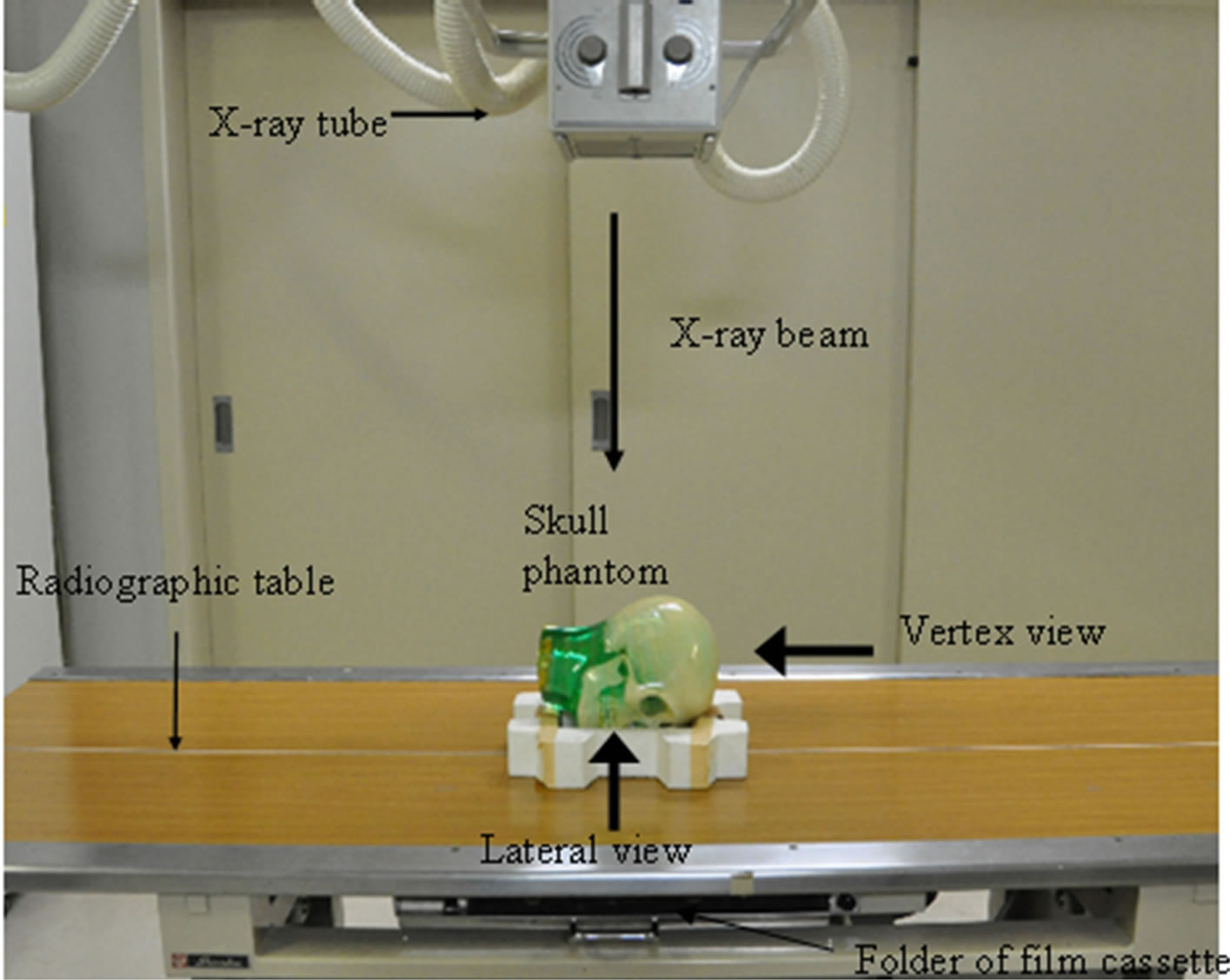
The optic canal is a tube with a diameter of approximately 5 mm through which the optic nerve passes. Radiography of the optic canal is used for the diagnosis of fracture in cases of traffic accidents and to determine the presence of infiltration by malignant tumors, such as orbital tumors, etc. The anthropological baseline that connects the infraorbital margin, the external acoustic meatus and the median sagittal line is used as a landmark for positioning. For the skull phantom, we used a sectional phantom (RS-108T; Radiology Support Devices (RSD), Inc.). As shown in Figure 1(a), the phantom is placed in the prone position for positioning practice. A radiological technologist observes the reference line from the lateral face of the phantom (lateral view, Figure 1(b)) and from the top of the head (vertex view, Figure 1(c)). The technologist observes the lateral and vertex views and positions the phantom to achieve adequate angles for both the angle between the anthropological base line and the film (α) and the angle between the median sagittal line and the film (β).
In order to represent the optic canal correctly, positioning is carried out so that the α angle becomes about 78 degrees and the β angle becomes about 55 degrees (Figures 2(a) and (b)). The axial of the optic canal is then perpendicular to the film plane. The image of the axial of the optic canal appears as a round projection in the orbital cavity, as shown in Figure 2(c) [7,8]. When the α angle is adequate and the β angle is about 40 degrees (Figure 2(d)) or about 70 degrees (Figure 2(e)), the image of the optic canal is not circular but elliptical. Moreover, the position of the image within the orbital cavity changes with different angles, and a difference in angles may cause an insufficient X-ray film image. Thus, a positioning technique that accurately adjusts the angles of the two reference lines is essential.
2.2. Development of a Training Tool
2.2.1. CT Measurement of a Phantom
In CT scanning, the phantom is usually placed in the supine position using a subsidiary implement so that the orbitomeatal (OM) line may be almost perpendicular to the bed, as shown in Figures 3(a) and (b). On the other hand, in positioning practice in optic canal radiography, the phantom is placed in the prone position with the face turned toward the film plane, as shown in Figure 3(c). The angle between the reference line and the film will be adjusted as described in Section 3 below. For CT, a GE Medical Systems Lightspeed16 was used in this study.
2.2.2. Construction of 3DCG Phantom
In order to produce a 3DCG phantom on the PC, CT image data of the phantom scanned in advance were used as 2-dimensional information and the number of slices was used as height information.
The 3DCG phantom of a skull is based on a cylindrical shape. That is, although the size of the transverse plane image is different, the overall contour can be expressed as an elliptical form. Additionally, the vertex of the polygon for approximating the contour was decided such that it might become an angle at almost equal intervals from the straight line that passes along the center of gravity. When the contour is approximated in detail, the vertices increase.
Twenty-seven slices were selected and the contour was approximated with a polygon. Figure 4 shows the construction of the 3DCG skull phantom. The two slices, Plane 1 and Plane 2, are shown in Figure 4(a). The trans-
 (a)
(a)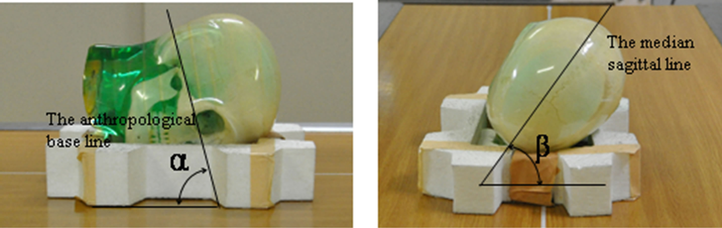 (b)
(b)
Figure 1. The X-ray tube and the skull phantom. (a) The X-ray tube and the skull phantom in positioning practice; (b) Lateral view: α is the angle between the anthropological line and the film cassette; (c) Vertex view: β is the angle between the median sagittal line and the film cassette.
verse plane images were converted to an 8-bit gray scale image, as shown in Figure 4(b). After binarizing the 8-bit gray scale image, the contours and center of the gravity were detected, and the intersection points of the contours and the line that passes along the center of gravity were obtained, as shown in Figure 4(c). Next, points P10, P11 … P1n were identified for Plane 1. Horizon line P10-P14 and perpendicular line P12-P16, which pass along the center of gravity, were drawn, as were straight lines P11-P15 and P13-P17, which divide the angle between the horizon line and a perpendicular line, and the coordinates of the intersections of the outline and each straight line were obtained. This process was repeated for Plane 2. By connecting these points with straight lines, a polygon approximating the contour was drawn, as shown in Figure 4(d). A wire frame model was then constructed based on connecting the nearest vertices between Planes 1 and 2, such as P10-P20 and P11-P21, as shown in Figure 4(e). A solid model was constructed by shading the surface defined by the wire, as shown in Figure 4(f). These procedures were carried out for the selected 27 CT slices. If a contour is approximated in detail, it is possible to produce the polygon by adding the straight line that follows the center of gravity and by increasing a vertex. Thus, when the approximated polygons of selected slices are stacked and the vertices are connected, the skull phantom is produced [9].
2.2.3. Production of the Plane Image
Two hundred or more transverse plane images of CT data
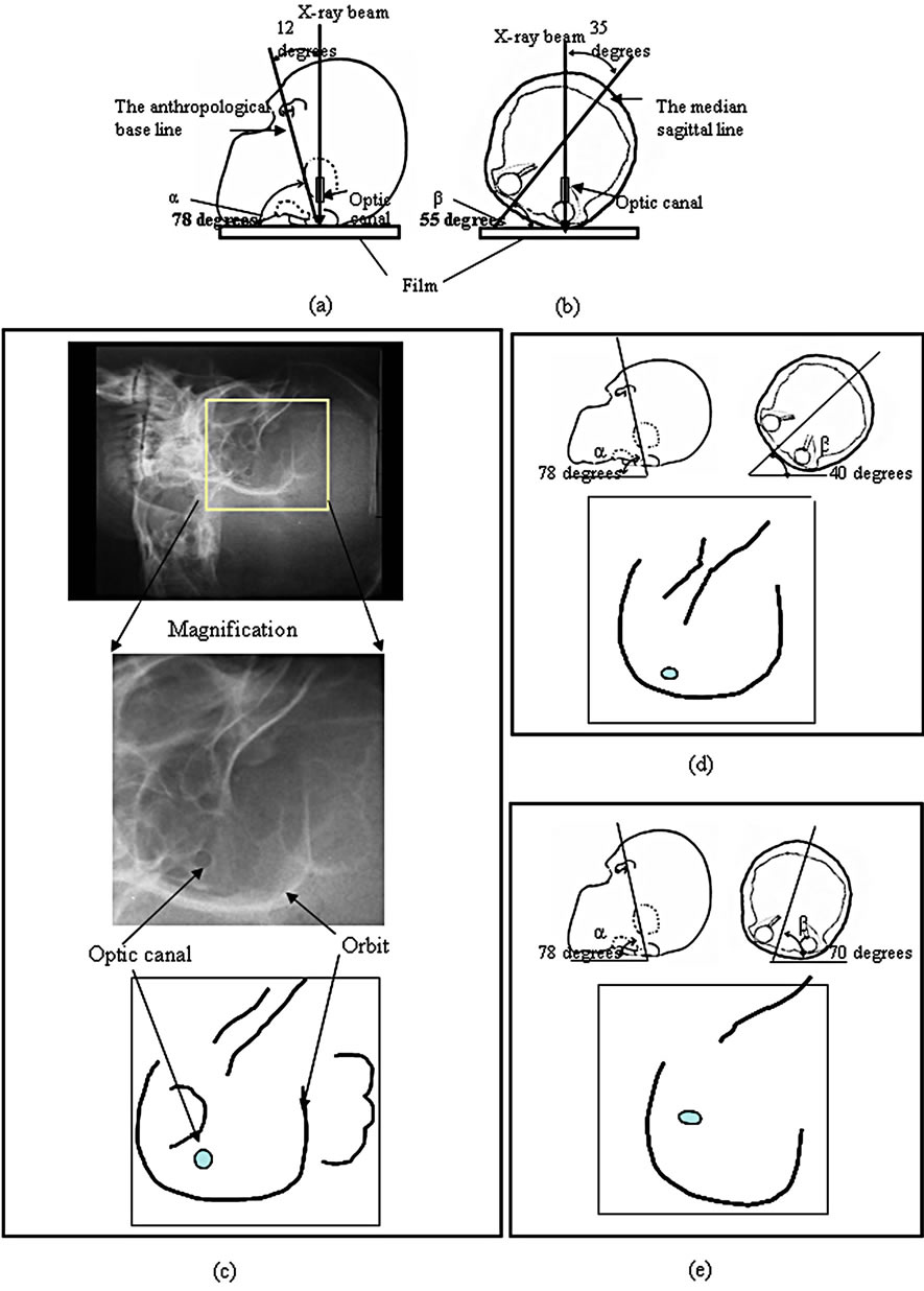
Figure 2. X-ray image and schemas of the left optic canal in the various position. (a) Lateral view; (b) Vertex view; (c) X-ray image and the schema of the X-ray image obtained by appropriate positioning; (d) Schema of X-ray image obtained by inappropriate positioning of the angle of between the median sagittal line and the film is about 40 degrees; (e) Schema of the X-ray image obtained by inappropriate positioning of the angle of between the median sagittal line and the film is about 70 degrees.
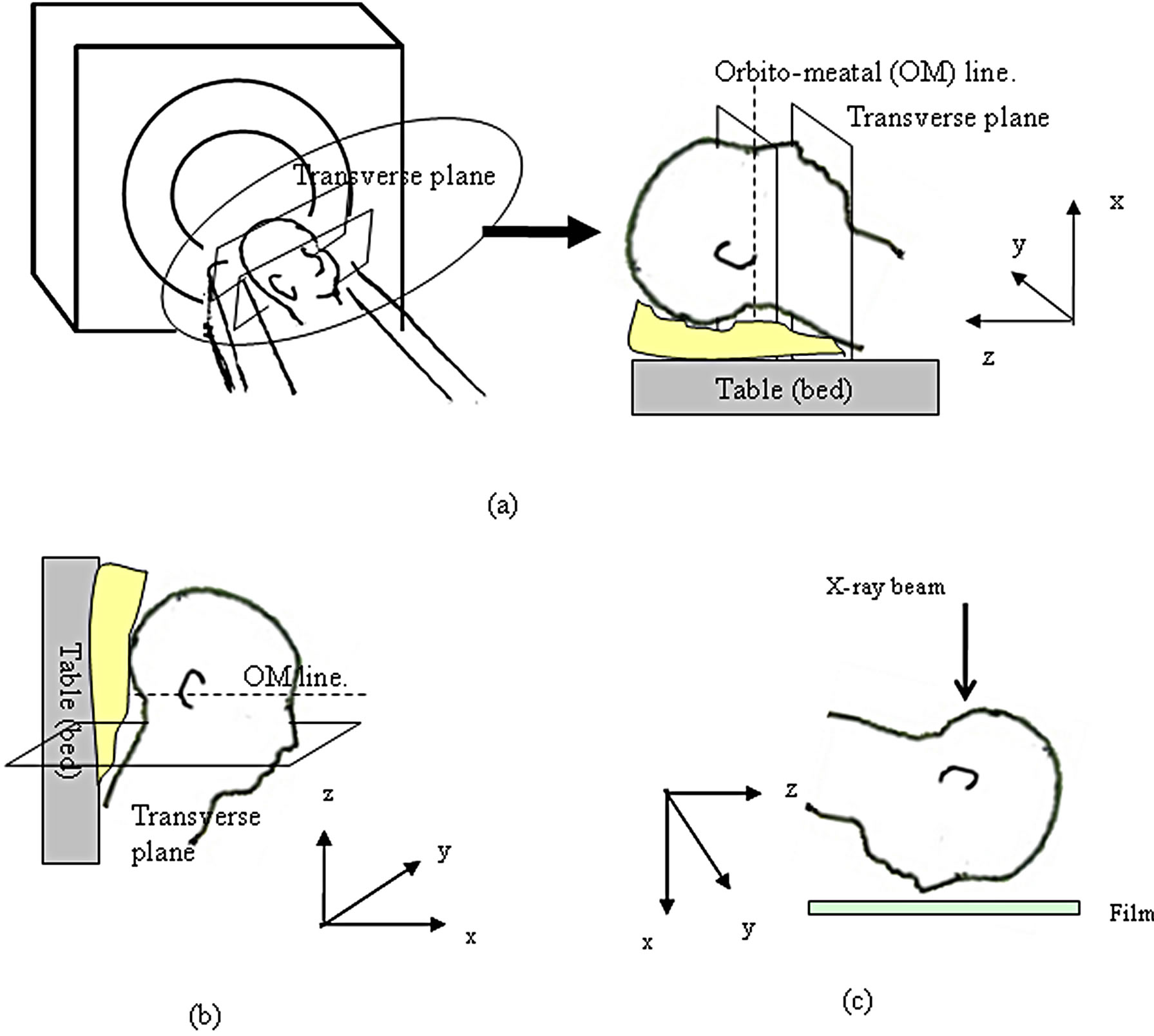
Figure 3. Positions of the skull phantom in the CT scanning and in the positioning practice. (a) Patient on the table in the CT scanning; (b) Lateral view in the CT scanning; (c) Lateral view in the positioning practice.
are used in order to produce the plane image. Figure 5 shows production process of the sagittal plane images and the new transverse plane images from the CT image data in order to correspond to the position of the phantom in the optic radiography. The CT image data is built by stacking the transverse plane images as shown in Figure 5(a). Di,j,k is the gray level at x = j and z = n − 1. m,  , and n represent the number of columns, rows and slices, respectively, in the x-, yand z-directions, and j, i and k represent arbitrary positions in x-, yand z-directions, respectively. First, the gray level images of CT data are rotated according to the angle of the reference line, and new sectional images are produced. The gray levels of the same row of each transverse plane image are extracted as shown in Figure 5(b). Extracted rows are arranged in order from z = 0 to z = n − 1 in z-direction and the gray levels are imaged as sagittal plane image as shown Figure 5(b). This process is carried out from y=0 to y=
 − 1 in each transverse plane image. The sagittal plane images are produced by processing all rows of each transverse plane image. The sagittal plane images are rotated so that the angle between the anthropological base line and the film becomes α as shown in Figure 5(c). Figure 5(d) shows the production process of new transverse plane image from sagittal plane images. The gray levels of the same line of each rotated sagittal plane image are extracted as shown Figure 5(d). Extracted lines are arranged in order from z = 0 to z = n − 1. The arranged gray level values are imaged and the new transverse plane image is produced. The new transverse plane images are produced by processing all lines of each sagittal plane image. The new transverse plane images are rotated so that the angle between the anthropological base line and the film becomes β as shown in Figure 5(e). In this way, the volume data of the gray level images corresponding to the determined position of the phantom.
Next, in order to observe the organ to be examined clearly in the projected plane image, the image is pro-
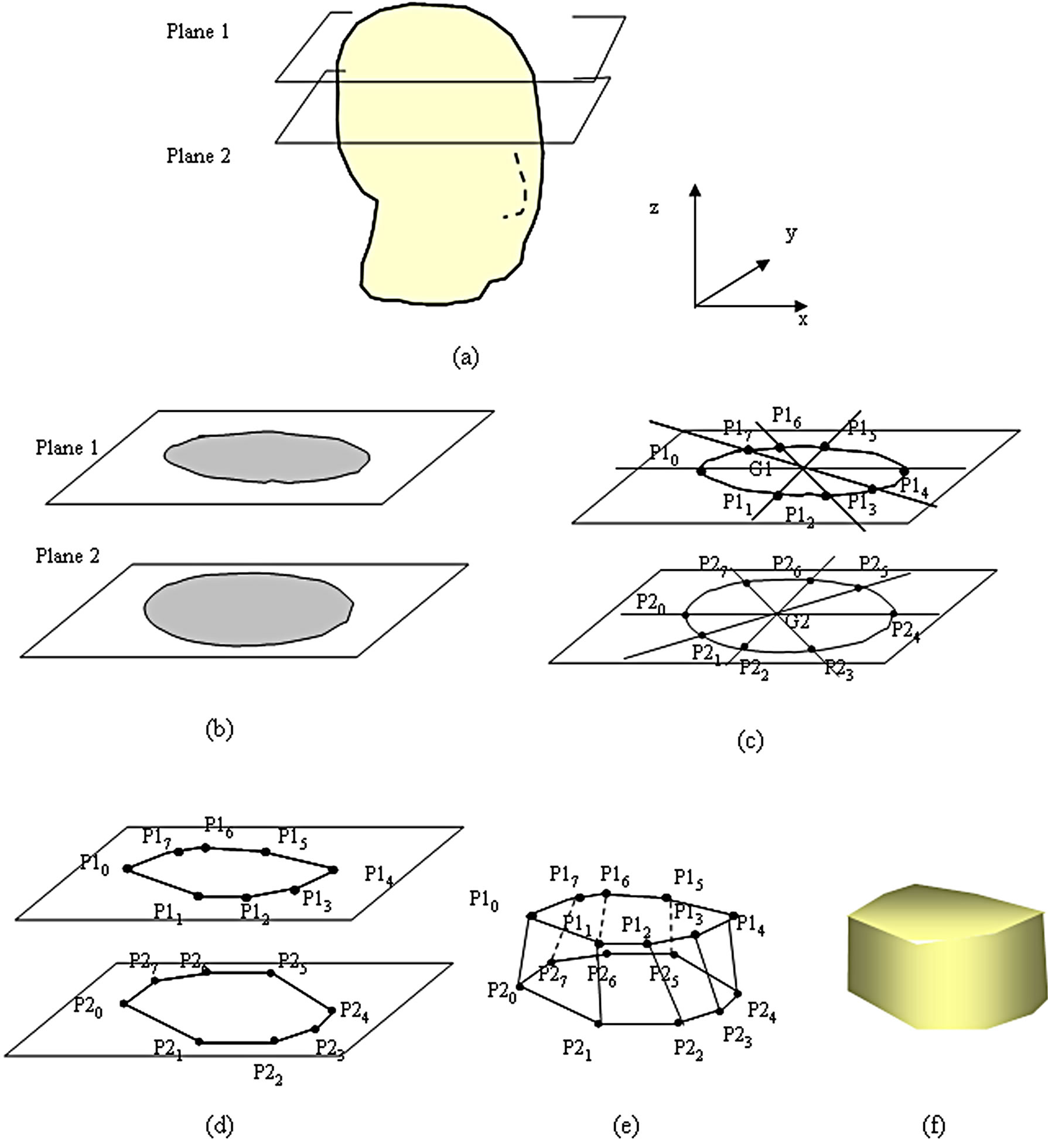
Figure 4. Production of the polygon and construction of the skull phantom from CT image. (a) Skull phantom image; (b) Grey scale image of transverse CT images; (c) Contours and the intersection of the lines passing through the center of gravity; (d) A polygon defined by many vertices; (e) Wire frame model; (f) Solid model.
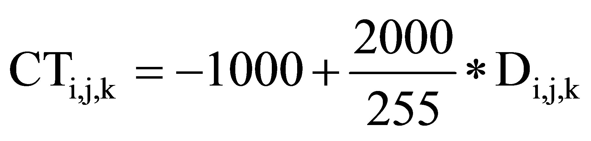
duced using attenuation coefficients μ and CT values. Since the relationships between the gray level image and CT values, and between CT values and attenuation coefficients, are defined, it is possible to convert the gray level image to CT values and attenuation coefficients. Figure 6 shows the process of the conversion from gray levels of the CT image data to attenuation coefficients [10]. First, the values of the 8-bit gray level image were changed to CT values using the following equation. Since the origin of the transverse-sectional image of a gray level Di,j,k is CT data, CT values CTi,j,k are calculated by Equation (1). The attenuation coefficient corresponding to each pixel of the traverse image can be calculated by Equation (2) from calculated CT values.
 (1)
(1)
 (2)
(2)
Equation (1) expresses the relationship between the gray level and the CT value. Equation (2) expresses the
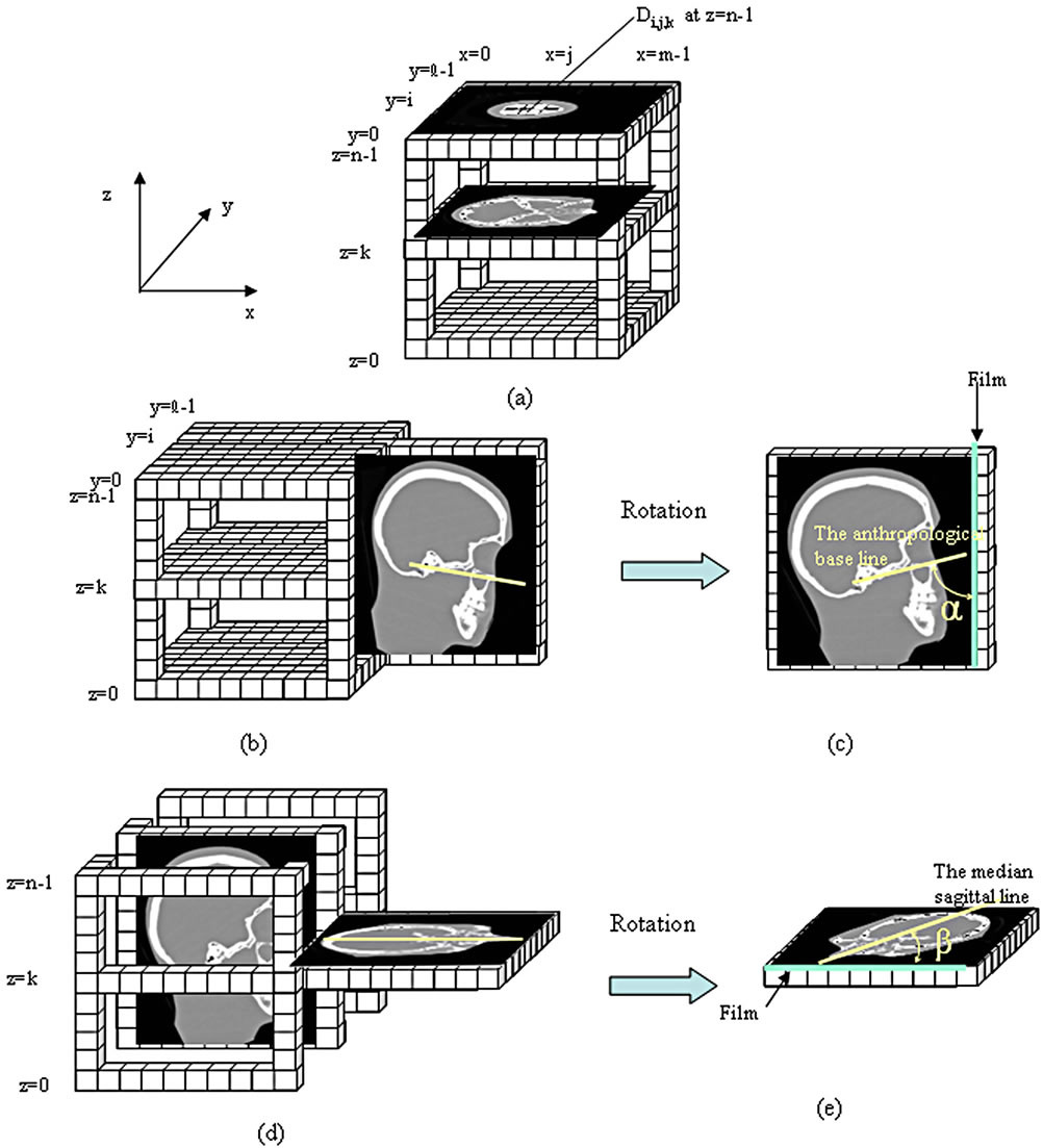
Figure 5. Production process of sagittal plane images and new transverse plane images from CT image data. (a) Transverse plane images; (b) Sagittal plane image; (c) Rotated sagittal plane image; (d) New transverse plane image from rotated sagittal plane images; (e) Rotated new transverse plane image.
relationship between the CT value and the attenuation coefficient .
.
In this study, when a tube voltage of 120 kVp was used on the CT scanner, the effective energy of the Xrays was about 70 keV [10]. Therefore, in Equation (2), 0.195 [cm−1] shows the attenuation coefficient of the water [11].
Figure 7 shows the addition of the attenuation coefficient and the plane image. Figure 7(a) shows the addition of the attenuation coefficient.
The added attenuation coefficient  is given by Equation (3)
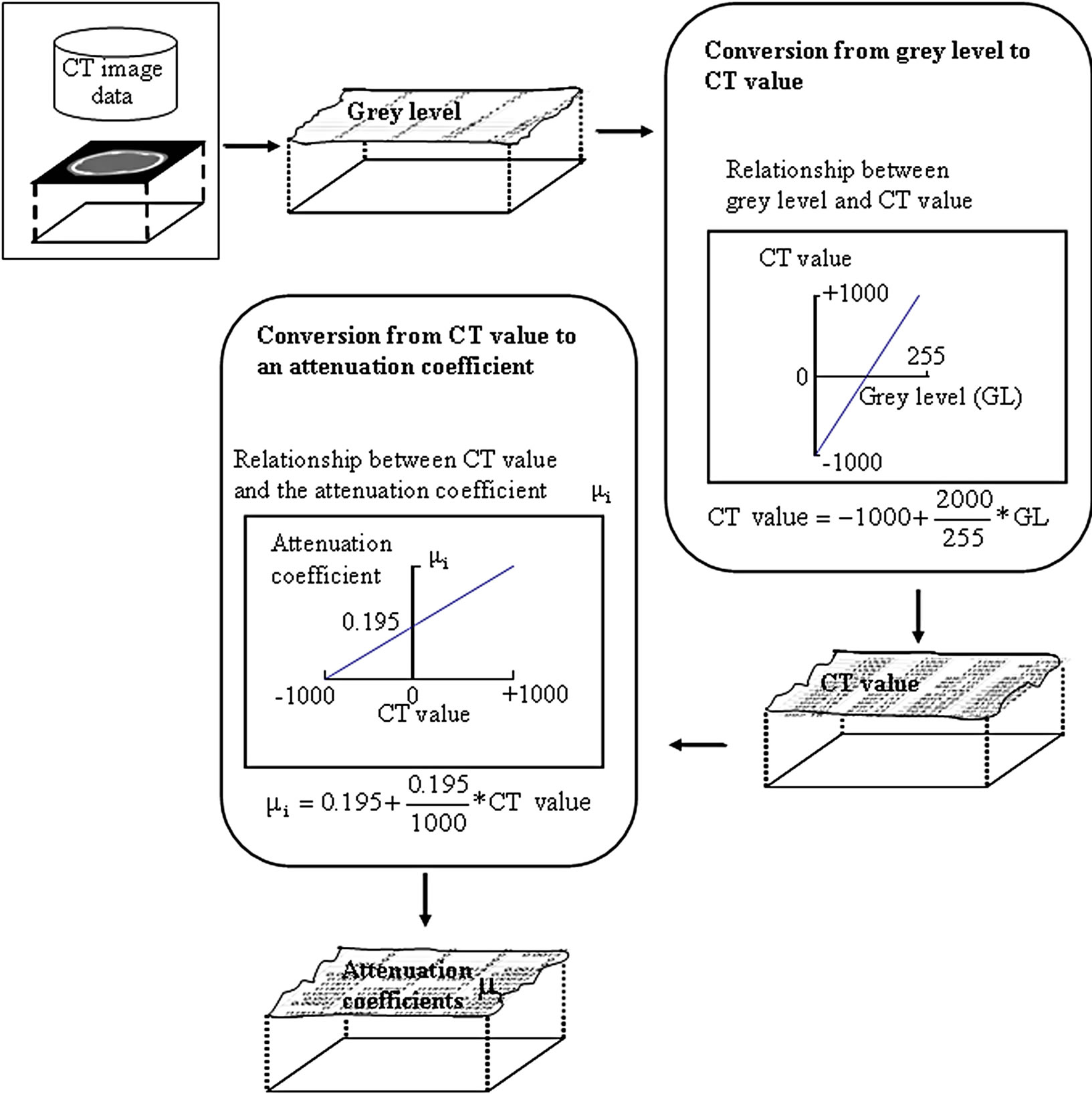
Figure 6. Process of the conversion from grey levels to attenuation coefficients.
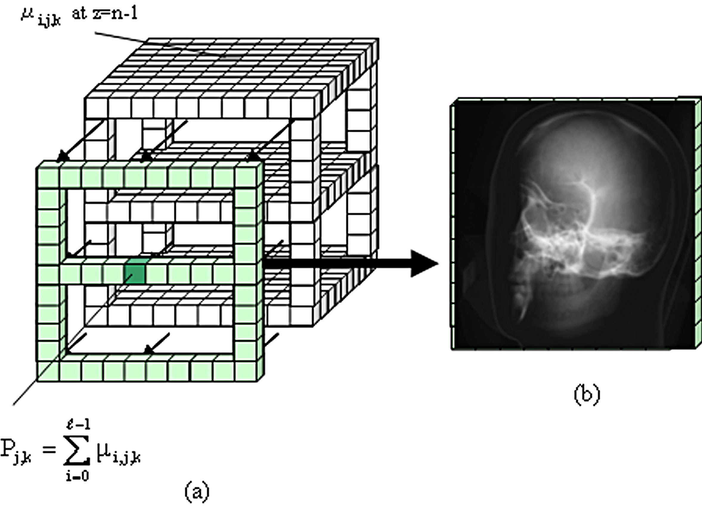
Figure 7. Procedure for obtaining a plane image from the CT data. (a) Addition of the attenuation coefficient in the projecting direction; (b) Plane image.
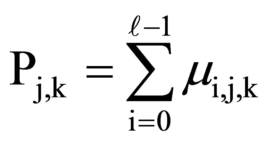 (3)
(3)
where  at x = j and z = k is the added attenuation coefficient from i = 0 to I =
  − 1. Each attenuation coefficient was added in the projecting direction of the X-rays, as shown in Figure 7(a). This process is carried out in order from z = 0 to z = n − 1.
The added attenuation coefficient correspond to the intensity of the penetrating X-ray beam. The projected plane image is produced by using this added attenuation coefficient by the method similar to the principle of image production of simple radiography [12]. The added attenuation coefficient of the penetrating air becomes the lowest and the gray level is thus at its minimum. The added attenuation coefficient of the penetrating bone becomes the highest and the gray level becomes the minimum. The conversion formula was set up such that the minimum and maximum densities correspond to 0 and 255 by gray level, respectively. In this way, the plane image at the determined position of the phantom is produced as shown in Figure 7(b).
3. Positioning Practice by Using PC
Figure 8 is a flow chart for positioning training. Figure 9(a) shows the situation in which the actual phantom in Figure 1(a) is replaced with a 3DCG phantom and positioning is performed on the PC. This training tool can change the viewpoint by mouse operation. A viewpoint is established for the X-ray equipment as shown in Figure 1(a), and the image seen from the upper part of the phantom can be obtained, as shown in Figure 9(a). Seeing the phantom from the vertex and lateral views makes it possible to accurately confirm the α and β angles.
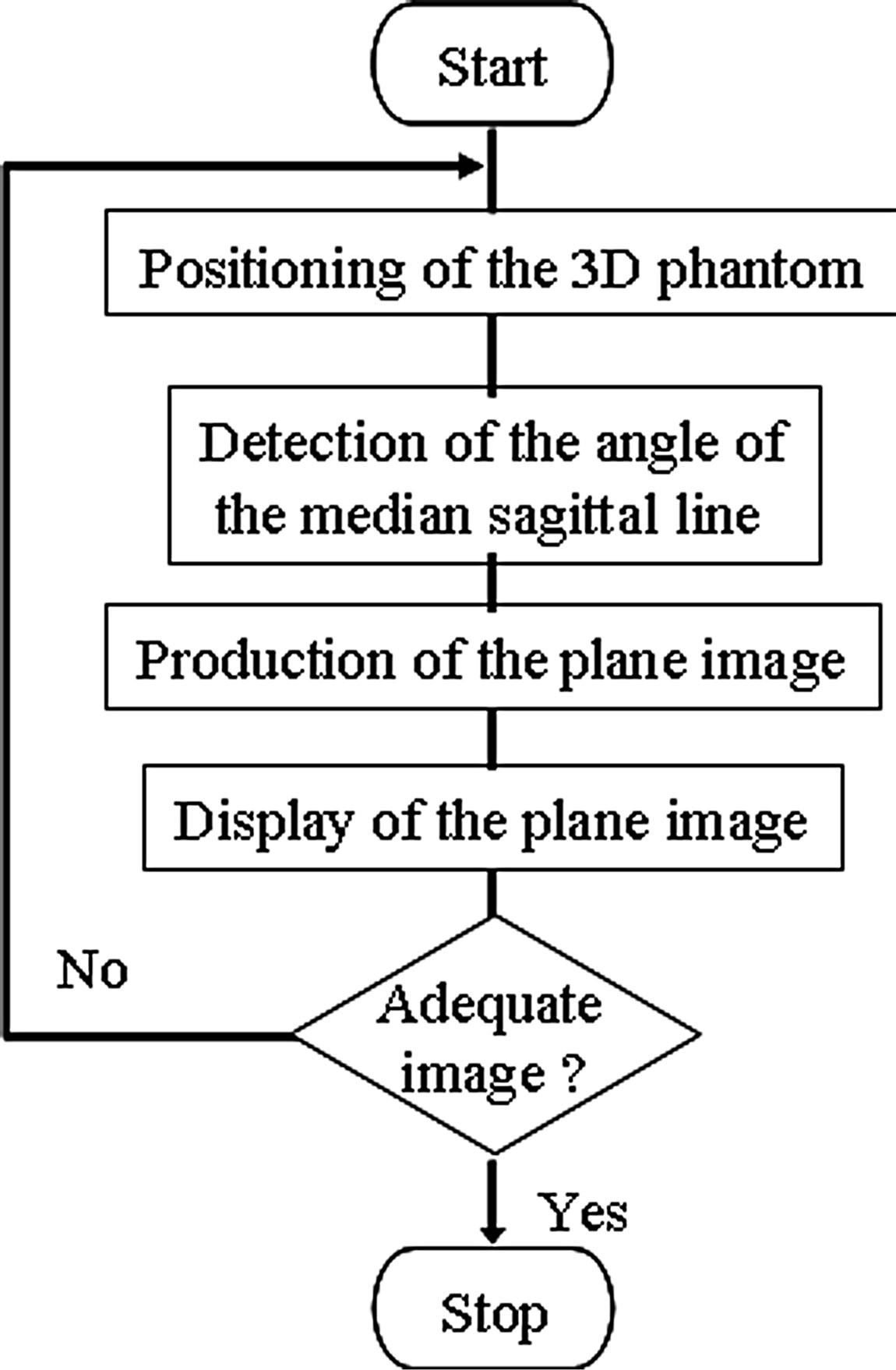
Figure 8. Flow chart for positioning training.
Moreover, with this training tool, the distance of movement and the rotational angle can be set up arbitrarily in one keyboard operation. Positioning is performed in the situation seen from the incidence direction of the X-ray beam. Although no landmark can be seen, it is important to be able to carry out positioning by imagining a reference line on the surface of the patient. 3DCG accumulates the x-y plane as a traverse CT image in the z-direction, as shown in Figure 5(a). In order to adjust the α angle in the lateral view, the phantom is rotated around the y-axis. In order to adjust the β angle in the vertex view, the phantom is rotated around the z-axis. Figures 9(b) and (c) show the figure seen from the lateral and vertex views, respectively, and the adjustment of the α and β angles by rotation.
Figure 10(a) shows the result of adequate angle positioning in left optic canal radiography. The positioning is carried out so that the α angle becomes about 78 degrees and the β becomes about 55 degrees. The 3DCG phantom is seen from the lateral view and from the vertex view in Figure 10(a). The plane image corresponding to positioning is displayed at the right. Figure 10(b) shows a magnified plane image on which the optic canal can be clearly seen.
Using our training tool, students can practice positioning any time and anywhere. If the student has poor anatomical knowledge, it will be difficult for that student to acquire adequate X-ray film images. This may make it necessary to repeat radiography, which imposes a burden on the subject. It is important for students to understand why a particular positioning and angle of the X-ray beam are required in any given situation.
The practical skills needed for the radiological technologist to tailor positioning to each subject’s individual differences are cultivated by considering the meaning of positioning. With a deeper understanding of anatomy, the landmarks of the subject can be imagined accurately, which in turn improves the student’s practical skills. Through the production of 3D models of all phantoms and the simulation of positioning, the relationship between anatomical knowledge and positioning technique is clarified. It is expected that training with actual X-ray equipment will be more efficient after the student has practiced with the training tool. Moreover, during the construction of the tool, CT images expressed as tomographic layers can be learned in three dimensions. Investigating the degree of rotation angle in traverse and sagittal images helps the student to achieve a deep anatomical understanding. Likewise, since CT data are threedimensional by stack and since projection images can be produced from all directions, the production of projection images is useful to understand the relationship between positioning and projection plane images; students can easily confirm differences in the projected plane image
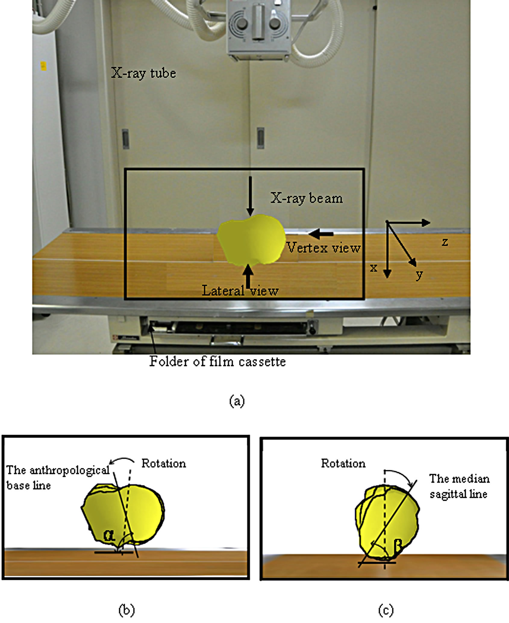
Figure 9. Positioning of 3DCG phantom by the training tool. (a) Direction of X-ray beam; (b) Schema of the rotation of the 3DCG phantom on lateral view. α is the angle between the anthropological line and the film cassette. (α is about 78 degrees); (c) Schema of the rotation of the 3DCG phantom on vertex view. βthe angle between the median sagittal line and the film cassette. (β is about 55 degrees).
corresponding to changes in the angle of the reference line. The student can repeat and practice various positionings using 3DCG phantoms of several body parts. By confirming the plane image corresponding to each position, the student will gain a greater understanding of the anatomical structure of the human body as well as a greater recognition of the spatial position of the organ to be examined.
Image media such as CG can be used to improve students’ understanding and memory, as well as to save time and create repeatability. The utilization of a widely used PC allows many students to practice at once. Moreover, since the plane image corresponding to positioning is easily produced, it can be confirmed immediately whether or not the positioning is adequate; learning is improved by this immediate feedback. It is expected that
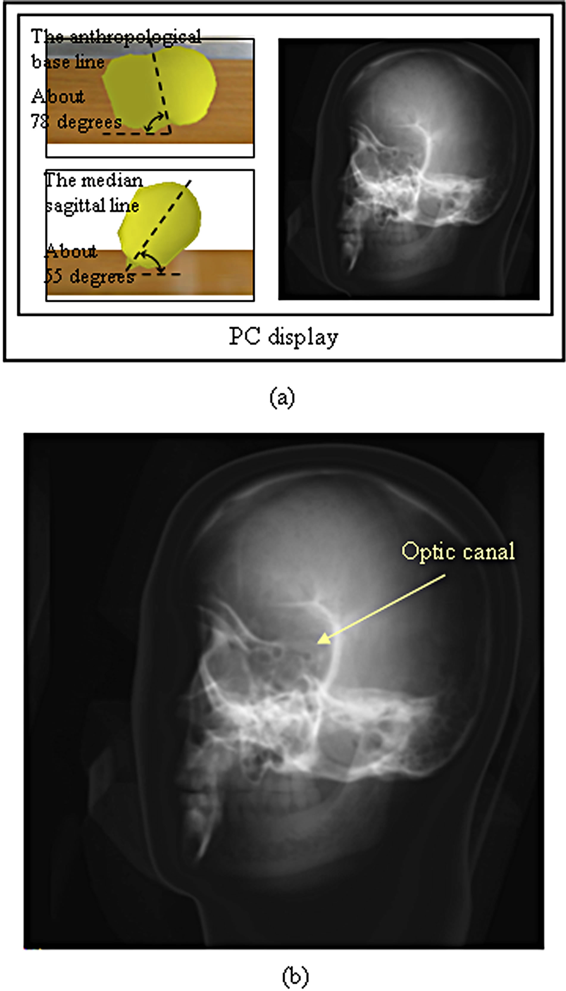
Figure 10. Positioning of the 3DCG phantom and the plane images of the left optic canal. (a) 3DCG phantom and its plane image. The phantom is rotated so that the angle between the anthropological baseline and the film cassette becomes about 78 degrees, and the angle between the medial agittal plane and the film cassette becomes about 55 degrees; (b) Final plane images of the optic canal.
training using our training tool will improve both positioning technique and the development of anatomical knowledge.
4. Conclusion
In this study, a training tool for acquiring positioning techniques in radiography was developed using a commercial PC and CT image data of a phantom. The 3DCG phantom was produced from CT data scanned in advance. The results obtained with the 3DCG phantom make it possible to position the phantom on the PC and calculate and display plane images corresponding to the positioning. Because this practice can be carried out without using actual X-ray equipment and plane images corresponding to all positioning can be produced, the tool is useful in helping students to understand the relationship between positioning and plane images. Construction of the anatomical structure of a human body is achieved by preparing 3DCG phantoms of several body parts during positioning training using a PC. This technique can be used to examine various organs, thus improving the student’s anatomical knowledge of each organ. A greater understanding of anatomy allows the radiological technologist to carry out positioning efficiently while taking into consideration any individual differences among subjects.
REFERENCES
- K. Inamoto, S. Beppu, et al., “Radiographic Image Technology,” Ishiyaku Publishers, Inc., Tokyo, 1997, pp. 37- 38.
- V. Merrill, “Atlas of Roentogenographic Positions, Volume One of Three Volumes,” The C. V. Mosby Company, Saint Louis, 1967, pp. 5-13.
- T. Maruyama and H. Yamamoto, “Study of Positioning Techniques for Skull Radiography,” Proceedings of the IEEE Instrumentation and Measurement Technology Conference, Sorrento, 24-27 April 2006, pp. 277-281.
- T. Maruyama and H. Yamamoto, “Study of Positioning Techniques for Skull Radiography Using CT Images,” Proceedings of the IEEE Instrumentation and Measurement Technology Conference, Warsaw, 1-3 May 2007, p. 7380
- T. Maruyama and H. Yamamoto, “Imaging Techniques for Radiography of Cervical Vertebrae Using CT Images,” Proceedings of the IEEE International Instrumentation and Measurement Technology Conference, Singapore, 5-7 May 2009, pp. 866-871
- T. Maruyama and H. Yamamoto, “CT Image Based Training Tool for Positioning in Radiography,” Proceedings of 2011 IEEE International Conference on Imaging Systems and Techniques, Penang, 17-18 May 2011, pp. 155-159. http://dx.doi.org/10.1109/IST.2011.5962172
- M. Nakamura, et al., “Radiographic Technique,” Iryoukagakusha, Tokyo, 2002, pp. 108-109
- R. A. Swallow, E. Naylor, E. J. Roebuck and A. S. Whitley, “Clark’s Position in Radiography,” ButterworthHeineman, Oxford, 1986, p. 210.
- S. Govil-Pai, “Theory and Practice Using OpenGL and Maya®,” Springer Science+Business Media, Inc., Boston, 2005, pp. 83-110.
- T. S. Curry III, J. E. Dowdey and R. C. Murry Jr., “Christensen’s Introduction to the Physics of Diagnostic Radiology,” 3rd Edtion, Lea & Febiger, Philadelphia, 1984, pp. 320-350.
- The Japanese Association of Radiological Technologists, “A Primer of Computed Tomography System,” Maguburosu Inc., Tokyo, 1977, pp. 21-44.
- J. H. Hubbell, “Photon Mass Attenuation and EnergyAbsorption Coefficients from 1 keV to 20 MeV,” International Journal of Applied Radiation and Isotopes, Vol. 33, 1982, pp. 1269-1290.