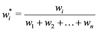
Positioning
Vol.1 No.1(2010), Article ID:3161,15 pages DOI:10.4236/pos.2010.11004
A Yield Mapping Procedure Based on Robust Fitting Paraboloid Cones on Moving Elliptical Neighborhoods and the Determination of Their Size Using a Robust Variogram
![]()
Technische Universität München, Lehrstuhl für Agrarsystemtechnik, Am Staudengarten 2, D-85354 Freising-Weihenstephan, Germany
Email: bachmai@wzw.tum.de
Received November 10th, 2009; revised August 21st, 2010; accepted August 25th, 2010
Keywords: Precision Agriculture, Yield Mapping, GPS, Elliptical Neighborhood, Paraboloid, Weighted Regression, Redescending M-estimate, Robust Variogram
ABSTRACT
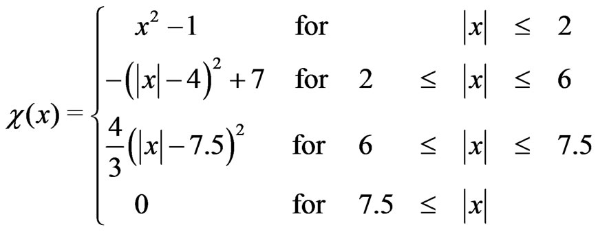
The yield map is generated by fitting the yield surface shape of yield monitor data mainly using paraboloid cones on floating neighborhoods. Each yield map value is determined by the fit of such a cone on an elliptical neighborhood that is wider across the harvest tracks than it is along them. The coefficients of regression for modeling the paraboloid cones and the scale parameter are estimated using robust weighted M-estimators where the weights decrease quadratically from 1 in the middle to zero at the border of the selected neighborhood. The robust way of estimating the model parameters supersedes a procedure for detecting outliers. For a given neighborhood shape, this yield mapping method is implemented by the Fortran program paraboloidmapping.exe, which can be downloaded from the web. The size of the selected neighborhood is considered appropriate if the variance of the yield map values equals the variance of the true yields, which is the difference between the variance of the raw yield data and the error variance of the yield monitor. It is estimated using a robust variogram on data that have not had the trend removed.
1. Introduction
The yield mapping method I extensively describe here follows Bachmaier [1] in many parts. It does not use filtering techniques to remove outlying yield measurements that are caused mainly by the monitoring process. According to Simbahan et al. [2], such errors include grain flow and other sensor errors (moisture, speed, swath width), errors due to geo-referencing and combine movement, operator errors and data processing errors (Shearer et al. [3], Blackmore and Moore [4]; Arslan and Colvin [5]). Steinmayr [6] gives a concise review of possible sources of error, their cause and impact and the corresponding filtering techniques (e.g. Thylén et al. [7,8], Noack et al. [9]).
The yield map values determined by my method does not depend on the removal of outliers, but from fitting the yield surface of the raw data using paraboloid cones on floating neighborhoods. By choosing these neighborhoods across the tracks wider than along them, the yield map can be adapted better to changes in yield along the tracks than across them. This is an advantage over other methods that often do not smooth sufficiently across the tracks. The parameters for modeling a paraboloid cone are estimated by robust weighted M-estimators (cf. Hampel et al. [10], Section 6.3) so that the influence of outliers is automatically restricted or completely annihilated. Therefore, discarding or downweighting values that deviate too much from a paraboloid yield surface around a neighborhood, as done by Bachmaier and Auernhammer [11], is not necessary. However, measurements that are wrong for technical reasons, such as values where the combine enters the harvest tracks, are assigned zero weight, which corresponds to removing them. The use of weights has the additional advantage that, contrary to all other filtering techniques in the literature mentioned above, there is no need to decide whether a measurement should be removed (weight 0) or not (weight 1). A measurement can be assigned any weight between 0 and 1, so the weights indicate how likely it is that the measurement is correct. In particular, there is no need to define limits for speed, moisture or swath width outside which the corresponding yield measurements should be discarded. The influence of a measurement on the yield map is greater, the greater its weight is. Only a measurement with weight zero has no influence at all, which corresponds to its being canceled.
The example in this paper uses a data set where the yields have been converted to dry matter yields. Time and header status were not measured. Therefore for every measurement the distance to preceding harvest paths was calculated. A distance that is considerably smaller than the cutting width of the combine indicates that the measurement cannot have come from a full swath, so it might be incorrect. The distance to preceding paths also downweights measurements because of end-path delays if the combine driver did not lift the header after harvesting a path. The GPS-points of the following low yield measurements are usually close to other harvest paths around the boundary of the field. I applied a smooth method of weighting to reduce the effect of such dubious measurements.
2. The Yield Mapping Method
2.1. Modeling Planes and Paraboloid Cones
A paraboloid cone (Figure 1) is modeled for determining a yield map value at  on a neighborhood around
  where only a measurement on
  can have full weight. The weights of other points within the selected neighborhood decrease smoothly to zero at the border of the selected neighborhood. These weights are called local weights, whereas those for downweighting dubious values are global weights.
Fitting paraboloid cones is only meaningful if one assumes that the true unknown yield surface is smooth. From a mathematical point of view, it should be a twice continuously differentiable function of the Gauss-Krüger coordinates. Fields where any rectangles were cut out, as often occurs in agricultural trials, are to be excluded from consideration.
But what is the true yield at a point of the field? Imagine a point as a 1 cm  1 cm square. One could say that if there is a wheat ear at this point, the yield (in Mg ha-1) is tremendously large (as the area of 1 cm2 is so small), whereas the yield is zero if there is no ear. Such a yield map would have a huge microscale variation, and that is not desirable. It is sensible that the true yield denotes the
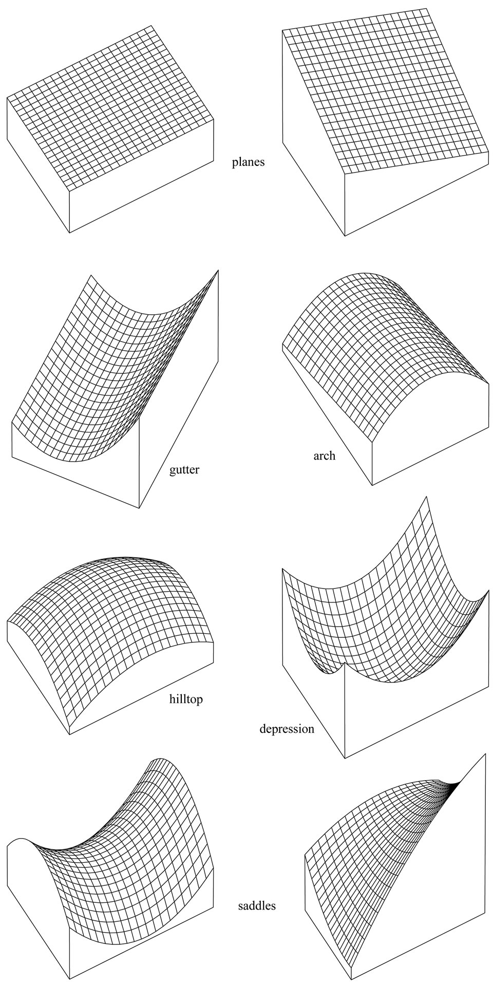
Figure 1. Planes and paraboloid cones obtained by the moldels in (3) and (1).
true average yield of a rectangle around this point, the rectangle to be harvested for measuring its yield with the monitoring process. Thus, the true yield surface is continuous. It has no microscale variation because points close to each other refer to almost the same area.
Every continuously differentiable function defined on a two-dimensional area can be approximated by a skewed plane if it is confined to a small environment. A paraboloid cone, however, approximates a twice continuously differentiable function better as it can also take account of hilltops or depressions. This allows a neighborhood that is considerably larger. Paraboloid cones arise from approximating smooth functions by a two-dimensional Taylor series that includes only linear and quadratic terms. Figure 1 shows some examples of what a paraboloid cone can look like.
The two-dimensional quadratic model for fitting paraboloid cones is

 (1)
(1)
where zi is the measured yield at the ith site . For reasons of numeric stability, the coordinates xi and yi should be the mean adjusted Gauss-Krüger coordinates
 (2)
(2)
where  and
and  are the means of the Gauss-Krüger coordinates
  and
and  over all points used for fitting the cone. The random variables
 ![]() in (1) denote the errors, which should be around zero.
in (1) denote the errors, which should be around zero.
In extrapolation or where there are few valid measurements around a point , the yield value should be obtained using a skewed plane rather than a paraboloid cone because the latter can lead to exaggerated values. A skewed plane is modeled by
 (3)
(3)
Such a plane is horizontal if .
.
2.2. Estimating the Coefficients of Regression by Redescending M-estimates
The regression coefficients are not estimated by classical least-squares because this method is not robust against outliers, which often occur in raw yield data. Instead, M-estimates are used.
2.2.1 The Concept of an M-estimate
To understand the concept of an M-estimate, consider first the simplest case of estimating a location parameter. A property of the mean ![]() is that the sum of deviations from it is zero:
is that the sum of deviations from it is zero: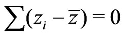 . This is demonstrated in Figure 2, where the bisecting line was moved back and forth until its deviations from the data points summed up to zero. Its intersection with the abscissa is the mean. Figure 2 shows that the outlier to the right causes the mean to move to the right.
This effect can be avoided by bounding the bisecting line, so that the influence of any outlier is also bounded. This is illustrated in Figure 3, where the bisector is replaced by a bounded function, ψ.
The influence of the outlier is reduced when solving
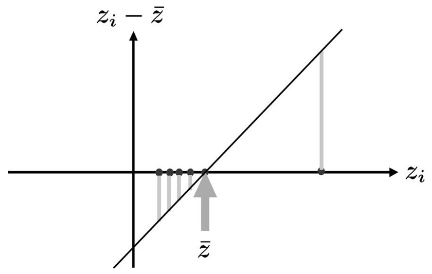
Figure 2. Deviations from the mean.
Figure 3. ![]() -values of deviations from an M-estimate
-values of deviations from an M-estimate![]() .
.
 . The solution of this equation,
 , which is the intersection of the ψ-function and the abszissa, is called an M-estimate. Figure 3 shows that if the largest value were shifted further to the right, it would have no influence, whereas the smallest value, which is not an outlier, retains its influence on the estimate. The latter would not apply if one computed a trimmed mean. An M-estimate whose ψ-function redescends to zero is called a redescending M-estimate, which removes the effect of large outliers completely.
Since the dispersion of the data is usually unknown, an M-estimate should be scale-invariant, which is so when a scale estimate is incorporated into the equation to be solved. The M-estimate for the location parameter is then defined by . The scale estimate
 can also be determined as an M-estimate for scale if one simultaneously solves an additional equation for
 . This will be done in the following, where M-estimates are expanded to a regression model.
2.2.2. Weighted M-estimates in the Regression Model
The objective is to estimate simultaneously the regression coefficients  and the scale parameter
 ![]() in (1) and (3) by robust weighted M-estimators. Thus,
in (1) and (3) by robust weighted M-estimators. Thus,  equations have to be solved, where
 ![]() is the number of regression coefficients (
is the number of regression coefficients ( if a skewed plane is modeled,
  if a paraboloid cone is modeled). The solutions
 ,
,  , and
, and  are the M-estimates for the unknown parameters
  and
and![]() . Following Huber [12] with slight changes for the scale estimate, the following system of equations is solved:
. Following Huber [12] with slight changes for the scale estimate, the following system of equations is solved:
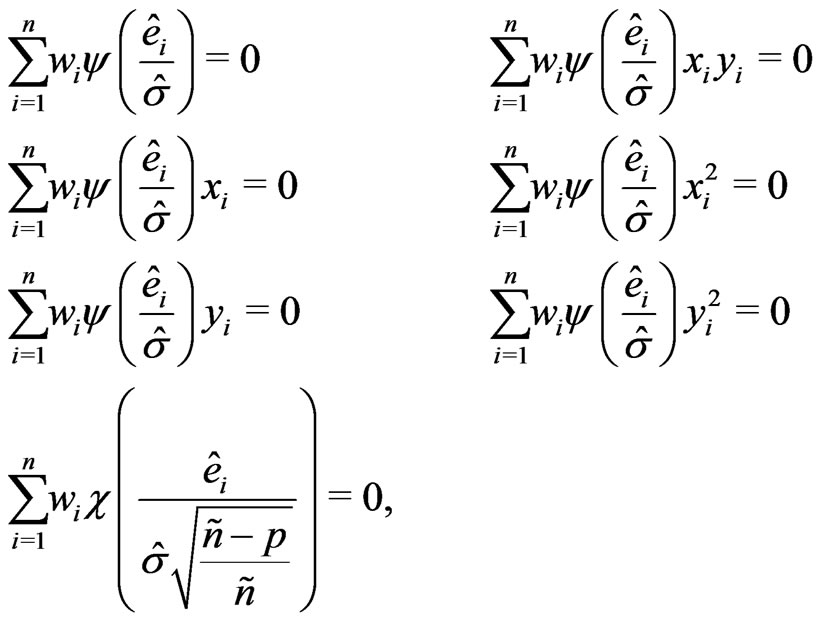 (4)
(4)
where the three equations of the right column in (4) are omitted for skewed planes ( ), and the residuals
 ![]() result as:
result as:
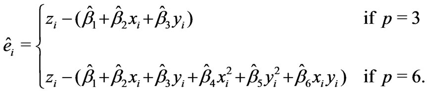 (5)
(5)
the weights  will be defined in (23). The number
 (6)
(6)
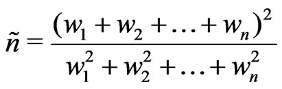
(Satterthwaite [13]) in the last line of (4) refers to them. I call it the effective number of data points. The idea behind this can simply be explained for the mean as a special case of linear regression. The variance of the mean of independent random variables  with identical variance
 is given by
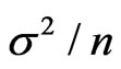 , but the variance of a weighted mean,
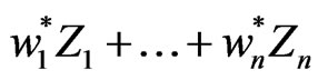 , where
 (7)
(7)
results in . Thus,
 ![]() data weighted according to
data weighted according to  lead to the same variance reduction as
  unweighted data. If all weights were equal,
 . The effective number
  is greater the more the weights
  equal each other. It is never greater than
![]() . Data points with a low weight,
. Data points with a low weight,  , such as those close to the border of the selected neighborhood, barely enlarge
 , unless there are no data points close to the point to be mapped.
The weighted M-estimates used for the regression and
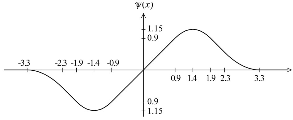
Figure 4. Redescending ![]() -function.
-function.
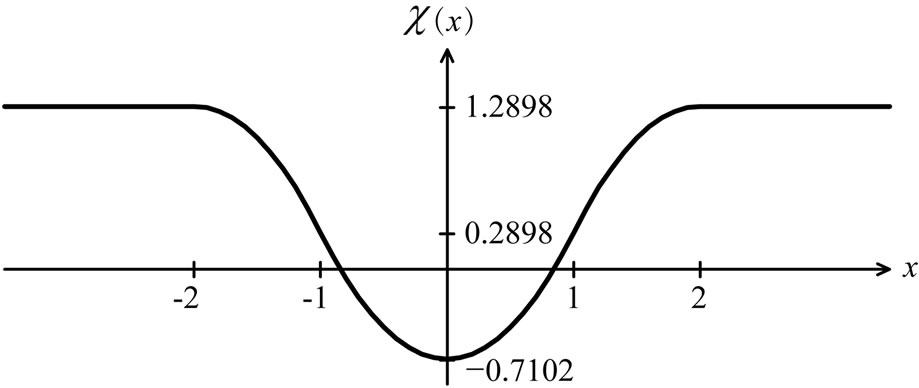
Figure 5. Bounded  -function monotone in
 .
.
coefficients,  , are based on the
  -function in (8) and the
  -function in (9). Illustrated are these functions in Figure 4 and Figure 5. Both
  and
and  consist of lines and parabolae only.
  is defined as
 (8)
(8)
and  is defined as
 (9)
(9)
where
 (10)
(10)
 ist the expected value of
  for an
  distributed random variable
 , thus providing the scale parameter
  for the standard normal distribution.
2.2.3 An Iterative Procedure to Obtain Regression Coefficients and Scale Estimate
To obtain the regression coefficients ,
,  , and the scale estimate
 , the equation system in (4) is solved in the following three successive steps:
First step: starting values
The starting value for the column vector of regression coefficients is obtained with the method of weighted least-squares:
 (11)
(11)
where the 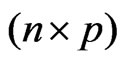 -matrix
 (12)
(12)
is the design matrix whose ith line ( ) consists of the line vector.
 (13)
(13)
which is based on the mean adjusted Gauss-Krüger coordinates xi and yi in (2). The weight matrix W = diag(w) is a diagonal matrix, i.e.  and
and  for
for .
.
The starting value for the scale solution is
 (14)
(14)
with  according to (7).
 , which has been defined in (6), should be considerably greater than
![]() . Since
. Since ![]() is based on squared deviations, it is subject to outliers, so that the robustly defined
is based on squared deviations, it is subject to outliers, so that the robustly defined ![]() might be overestimated. However, large starting values for scale should be preferred as they counteract the danger of scale implosion (Huber [14]).
might be overestimated. However, large starting values for scale should be preferred as they counteract the danger of scale implosion (Huber [14]).
Second step: iteration based on  and
and ![]()
The classical starting values obtained in the first step,  in (11) and
  in (14), serve as the results of the iteration
  in the second step.
To avoid solutions that could abduct us from the bulk of the data, redescending M-estimates are not yet applied in the second step when running the iteration procedure, which will be described soon. Instead, the  -function
  in (8) is made monotone by replacing its redescending parts by horizontal lines:
 (15)
(15)
The -function remains unchanged, as it is already monotone in
 .
.
Third step: iteration based on  and
and 
Finally, the same iteration procedure is run again, using the results of the second step as starting values (iteration ) and applying the redescending
  -function
  in (8) instead of the monotone one in (15). The results of the last iteration,
  and
and , are the numerical solutions,
 and
and , of the equation system in (4).
The iteration procedure
The iteration procedure follows Huber [14] or Huber [12], Section 7.8. However, contrary to Huber, the M-estimates ,
, , and
, and  in (4) are weighted, and the definition of
  slightly differs from that of Huber. Therefore, the pocedure needs to be changed accordingly.
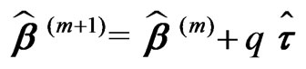
It suffices to describe the (m + 1)th iteration on the basis of the results of the mth iteration ( ):
):
Based on the vector of regression coefficients ![]() of the mth iteration, the residuals are computed first:
of the mth iteration, the residuals are computed first:
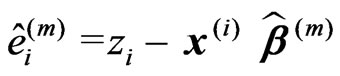 (16)
(16)
Then the ![]() -estimate of iteration
-estimate of iteration  is calculated:
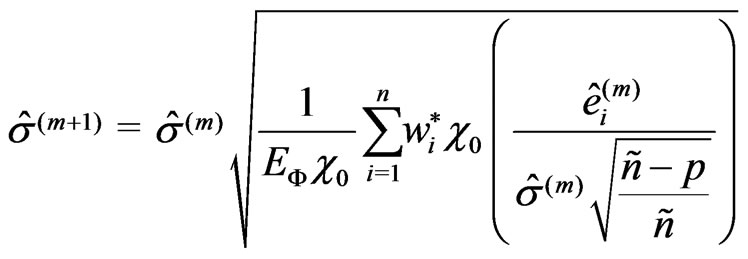 (17)
(17)
with  according to (7). Now, the residuals
  are used to compute the so-called Winsorized residuals:
 (18)
(18)
where  in (15) if the iteration refers to the second step, and
  in (8) if it concerns the third step.
Using the vector of these Winsorized residuals,  , the difference vector
 (19)
(19)
is calculated by weighted least-squares and used to compute the new vector of coefficients of regression:
 (20)
(20)
According to Huber [12], p. 183, theoretical considerations suggest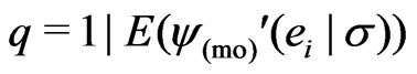 . For
. For distributed
 , this yields
 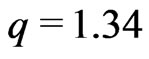 if
if , and
, and  if
if . Empirical results showed that the factor
  could be relaxed, but only because the
  -functions used are normed such that
  on a large area around 0.
The iteration procedure ends if
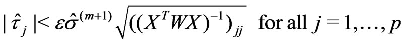
 (21)
(21)
for a small , e.g.,
  in the second and
  in the third step;
  is the j th diagonal element of
 .
.
2.3. Weights
2.3.1. Global weights
The most important reason for omitting yield monitor data concerns start-path delays (see e.g. Thylén et al. [7], Simbahan et al. [2]). The first ![]() measurements are given the global weight zero, which discards them; the (m + 1)th measured value is downweighted by a factor of 0.5 because of uncertainty as to whether this value is correct. The other values are then weighted fully in the context of delays. The size of
measurements are given the global weight zero, which discards them; the (m + 1)th measured value is downweighted by a factor of 0.5 because of uncertainty as to whether this value is correct. The other values are then weighted fully in the context of delays. The size of ![]() depends on the yield monitor. For the Claas Agrocom Quantimeter, which was used in the trial described here,
depends on the yield monitor. For the Claas Agrocom Quantimeter, which was used in the trial described here,  proved adequate.
Another reason for downweighting values is if the GPS points of the current swath are close to a preceding neighboring swath. Such a small distance might arise from GPS errors or inaccuracies, but it can also be the consequence of a smaller current swath width. If the minimum distance to the preceding harvest tracks, , is small, it is less likely that the measured yield comes from a full swath width. At present, a raw yield value is weighted fully (weight 1) only if
 , whereby sw means the “full” swath width, which is somewhat smaller than the combine’s cutting width, cw, when the combine is steered by a man. If
 , the raw yield value gets weight zero. The weights in between are obtained by linear interpolation. This is illustrated in Figure 6.
In Bachmaier [1], the interpolation interval was 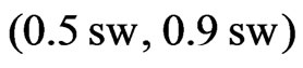 instead of
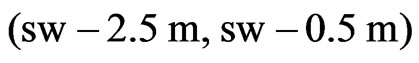 , whereby I was influenced by researchers who discarded yield measurements with
 . I no longer defend this because the positioning system’s accuracy, which is the main source of variation of
 , does not depend on the combine’s cutting width, cw, to which the full width of a swath, sw, is closely related. However, if positioning errors can be assumed to be approximately normally dis tributed, the left half of a Gaussian bell curve,
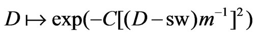 , could give a still more suitable downweight function for
 . For,
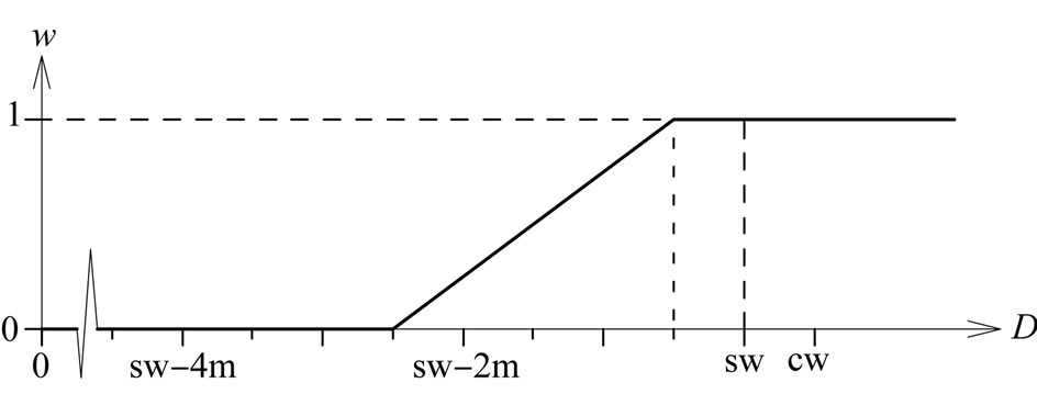
Figure 6. A weight factor  as a function of the minimum distance
  to the preceding harvest tracks.
 , it comes close to the function in Figure 6.
The global weight, , is the product of the single weight factors. For example, if the measurement is the
  value of a harvest track, it is downweighted by a factor of 0.5, as mentioned above, and if its minimal distance from neighboring tracks,
 , is
, is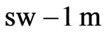 , it results in a weight factor of 0.75 (Figure 6). Finally, the yield at this point is given the global weight
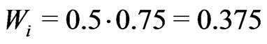 .
.
Other sources of error that result in dubious measurements, e.g. unusual values for moisture or speed, could be dealt with similarly. The greater the likelihood that the measurement is erroneous, the lower its weight is.
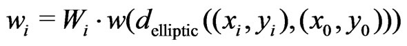
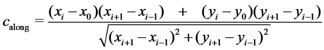
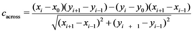
2.3.2. Local Weights Based an Elliptical Distance from 
To estimate the regression coefficients for the paraboloid cone or the plane at the point , all points
  within an elliptical neighborhood see Figure 7 are considered. The local weight 1 holds only at
 , whereas the weight is zero at the boundary of the selected neighborhood. The transition in between is obtained by quadratic interpolation, because a local deviation corresponds to a position error, and errors are usually quadratically considered. In particular, the local weight function is defined as
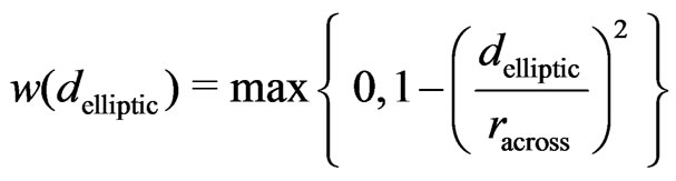 (22)
(22)
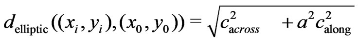
where  denotes the radius of the neighborhood across the tracks and
  is a distance measure between
  and
and  on the basis of an elliptical metric, which will be defined in (24). The weights
  are local because they depend on the distance from the fixed point
 , and they change if this point changes.
The global weights, , do not depend on
 . The final weights,
 , of the yield measurements at the points
  within the neighborhood for determining the regression coefficients in (4) are the products of the global and local weights, so they also depend on
 :
:
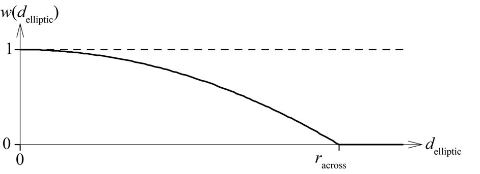
Figure 7. Local weight functions ![]() and
and ![]() for regression coefficients and scale according to (4).
for regression coefficients and scale according to (4).
 (23)
(23)
In Bachmaier [1] I used different local weight functions, ![]() and
and![]() , and thus, different weights,
, and thus, different weights,  and
and![]() , in the equation system in (4), where the former served to estimate the regression coefficients
, in the equation system in (4), where the former served to estimate the regression coefficients  by means of the
  -function, and the latter were used to estimate
 ![]() by means of the
by means of the  -function. The weight function
  decreased linearly from 1 to 0, whereas
 ![]() downweighted more slowly (with the fourth power) to increase the effective number of data points with respect to the scale estimate, because higher moments — the scale estimate is a second moment — require more data to be efficient enough. However, since the weights
downweighted more slowly (with the fourth power) to increase the effective number of data points with respect to the scale estimate, because higher moments — the scale estimate is a second moment — require more data to be efficient enough. However, since the weights , which were used to estimate the regression coefficients, decreased faster to 0, the paraboloid cone was less forced to adapt to yield values close to the neighborhood’s border, and hence, larger residuals could arise that distort the scale estimate. Therefore, and for the sake of simplicity, I now use the same local weight function, the quadratically decreasing
 ![]() in (22) Figure 7, and thus the same weights
in (22) Figure 7, and thus the same weights  for estimating both
 ,
,  , and
, and![]() .
.
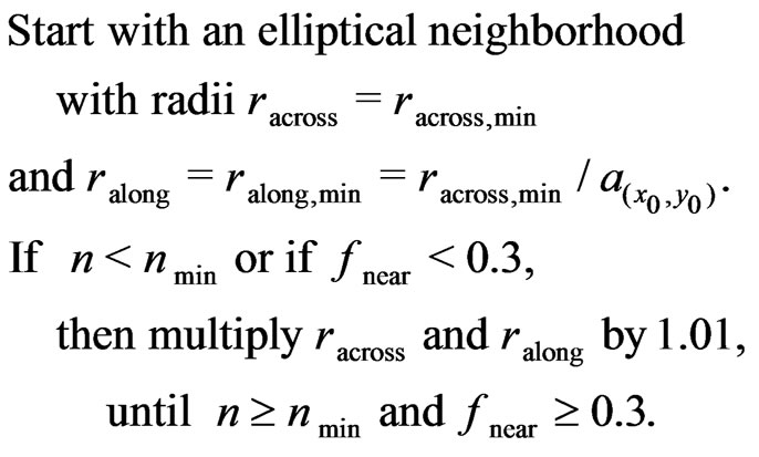
2.4. An Elliptical Neighborhood
Raw yield data often show surface textures along the harvest tracks that remain when the data are amended. In Bachmaier and Auernhammer [15] I showed that ordinary kriging of amended data did not smooth out the harvest tracks sufficiently. Therefore, the neighborhood on which the paraboloid yield surface is fitted should be wider across the harvest tracks than it is along them. This can be achieved by an elliptical neighborhood Figure 8.
The butterfly neighborhood I used in Bachmaier [1] is more appropriate as a filtering technique (Bachmaier and Auernhammer [11]), because its length along the tracks is a little shorter at the current track than it is at the two adjacent tracks, and the assessment of a yield value (correct or not) should less be affected by values of the same track; they could be erroneous as well, for example if the swath has not its full width.
A single swath of wrong values can also distort a yield estimate if its influence on the paraboloid regression is
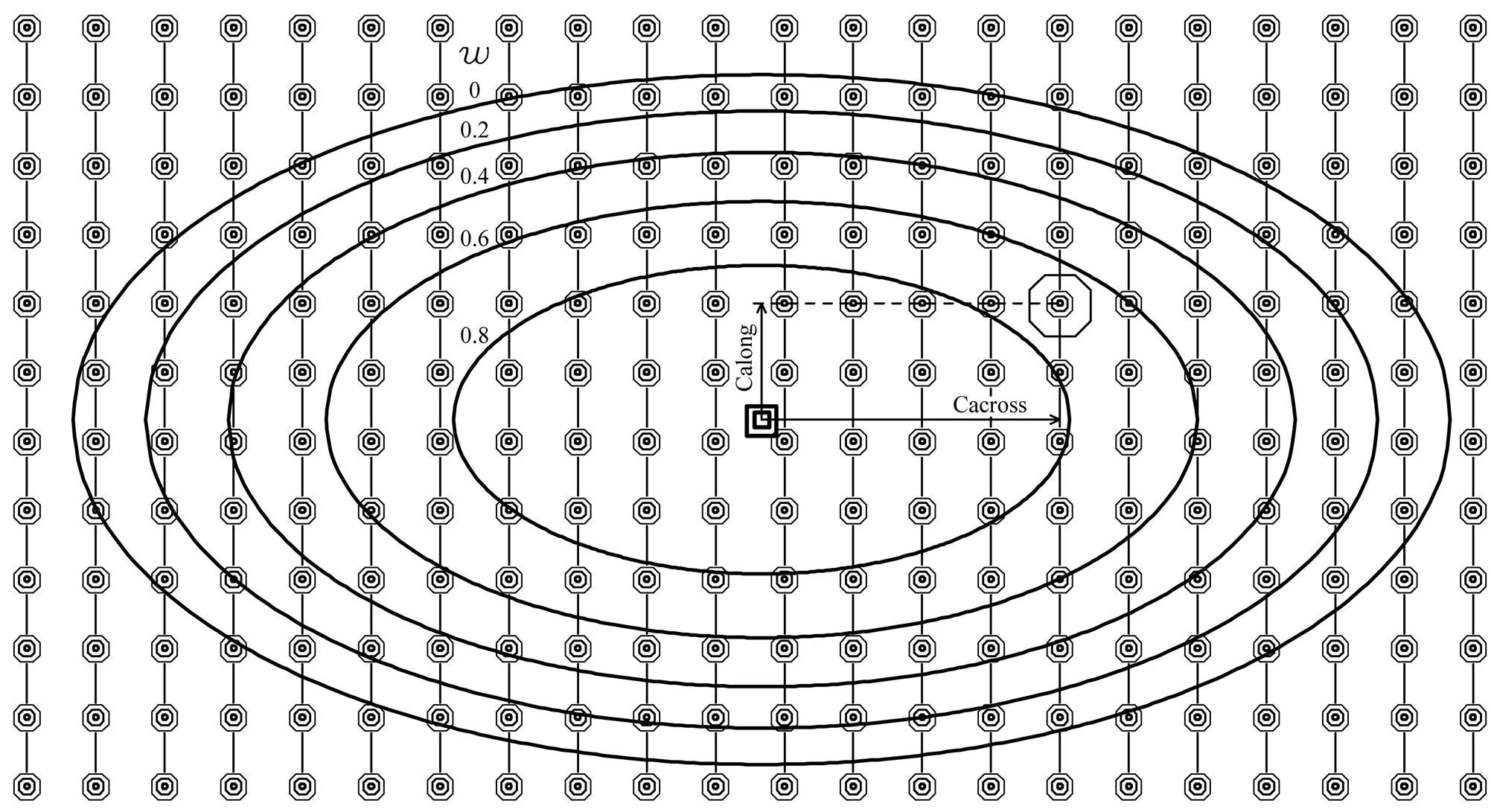
Figure 8. Contour lines of the weight function  in (22) on a map point’s elliptical neighborhood with
  and
and , i.e.
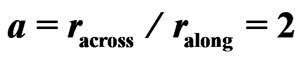 , at a quadratic pattern of measuring-points.
too large. To avoid this, the neighborhood must be chosen large enough, and the tracks in the mid should have nearly the same sum of weights . This is a further reason why the chosen local weight function
 ![]() defined on an elliptical neighborhood downweights more slowly than linearly.
defined on an elliptical neighborhood downweights more slowly than linearly.
The ‘elliptical metric’,  , is based on the ratio,
 ![]() , of the ‘radius’ (half diameter) of the ellipse across the harvest track and the ‘radius’ along it:
, of the ‘radius’ (half diameter) of the ellipse across the harvest track and the ‘radius’ along it:
 (24)
(24)
The components of the difference vector
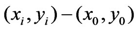 along and across the harvest tracks,
  and
and , can be calculated from neighboring GPS points on the same harvest tracks as follows:
 (25)
(25)
2.5. Rules for Deciding on the Model and the Elliptical Neighborhood’s Size and Shape
2.5.1. Advantages and Disadvantages of Modeling Planes and Paraboloid Cones
The main advantage of modeling paraboloid cones over planes relates to yield peaks or depressions see Figure 1. If the yield is fitted by planes, a depression is overestimated and a peak is underestimated, whereas a paraboloid cone fits optimally provided that the neighborhood is not too large. Nevertheless, modeling paraboloid cones can lead to exaggerated results in the case of extrapolation. This can occur at the beginning of a swath width and along the edges of a field, and extrapolation can be based on points far away from . Therefore, where the extrapolation is over a distance or where there are few measurements near to
 , the skewed plane should be used.
2.5.2. The Measure
The choice of model can be based on the ratio of the sum of weights within a narrower neighborhood around  to the sum of weights within the entire neighborhood. A small ratio indicates that there are only a few valid measurements close to
 , so the desired fit is determined mainly by extrapolation. The paraboloid cone should be used only if this ratio exceeds a certain value.
The considerations that lead to the choice of an elliptical neighborhood also depend on a sufficiently large share of valid measurements within the nearer environment. If it is too small, a circular neighborhood should be used.
To ensure that the ratio changes smoothly, a function for a degree of membership in the narrower environment is used, which is 1 at the point . Likewise to the local weight function
 ![]() in (22), it decreases quadratically to zero at the boundary of the neighborhood because the effect of a paraboloid extrapolation can also increase quadratically with the distance. This leads to the definition of the following ratio:
in (22), it decreases quadratically to zero at the boundary of the neighborhood because the effect of a paraboloid extrapolation can also increase quadratically with the distance. This leads to the definition of the following ratio:
 (26)
(26)
The sums relate to the weights of all points  within an initial elliptic neighborhood of
 . An increase of its size according to the rule in (30) does not involve a new computation of
![]() .
.
To form an idea of the limits at which to model paraboloid yield surfaces or at which to use an elliptical neighborhood, the ratio of the expected values of the nominator and the denominator of![]() is helpful. Under the assumption of continuously and uniformly dispersed data points with global weight
is helpful. Under the assumption of continuously and uniformly dispersed data points with global weight , this ratio does not depend on the radii of the ellipse, so it can be calculated for a circle with radius 1:
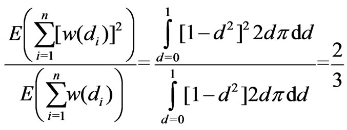 . (27)
2.5.3. Determining the Proportion of the Radii of the Elliptical Neighborhood
Since monitor yield data often show surface textures along the harvest tracks, an elliptical neighborhood that is wider across the tracks than it is along them is preferred. The determination of an adequate radius proportion,  , with statistical methods is not afforded in this article. Yield data obtained with the Claas Agrocom Quantimeter suggest that
 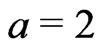 could be a good choice. However, if there are few values in the nearer environment of
 , so that
 ![]() in (26) is small, the neighborhood should not be shortened along the tracks, and a circular neighborhood, i.e. a local radius ratio of
in (26) is small, the neighborhood should not be shortened along the tracks, and a circular neighborhood, i.e. a local radius ratio of , should be used. Yet to determine this
![]() , an initial neighborhood is already necessary. It is based on the `full' radius ratio,
, an initial neighborhood is already necessary. It is based on the `full' radius ratio,![]() , and on an initial radius
, and on an initial radius , a proper value of which can be found using the method in Section 3. The initial radius along the tracks is then given by
 . Based on this neighborhood, an initial measure,
  in (26), is computed to determine the local radius ratio
 . For
. For it is assigned its maximum value,
  , because 0.6 is already close to the ratio,
 ![]() , of expected values in (27). A circular neighborhood, i.e.
, of expected values in (27). A circular neighborhood, i.e. , is only used if
 , and for
  the local radius ratio,
  , is defined as a linear interpolation between 1 and
![]() . This is summarized in the following definition:
. This is summarized in the following definition:
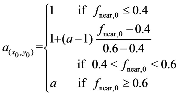 (28)
(28)
Further computations of ![]() are based on a neighborhood that already respects this local radius ratio,
are based on a neighborhood that already respects this local radius ratio, . When deciding on the model, the radius
  of the ellipse remains unchanged, but the radius along the tracks is adapted to it:
 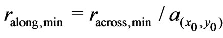 .This can enlarge the neighborhood, but it rarely occurs, unless corners of a field are harvested. The elliptical neighborhood with these radii,
  and
and , also serves as the initial neighborhood in (30), where the final neighborhood size is determined. Its shape, however, i.e., its radius ratio,
  , remains unchanged, until the next point
  is mapped.
2.5.4. The Decision on the Model
Paraboloid cones are preferred, therefore, the limit at which to model it should be less than the ratio in (27). The transition from planes to paraboloid cones should be smooth to obtain a continuous yield map. In Bachmaier [1], where both the local weight function and the degree of membership in the narrower environment decrease linearly, the ratio of expected values of nominator and denominator of ![]() resulted in 0.5, and a transition interval of (0.35,0.45) has proved adequate. Considering that this ratio has resulted in
resulted in 0.5, and a transition interval of (0.35,0.45) has proved adequate. Considering that this ratio has resulted in ![]() for weight and membership quadratically decreasing, a transition area of (0.5,0.6) appears appropriate. This leads to the following model decision in (29):
for weight and membership quadratically decreasing, a transition area of (0.5,0.6) appears appropriate. This leads to the following model decision in (29):
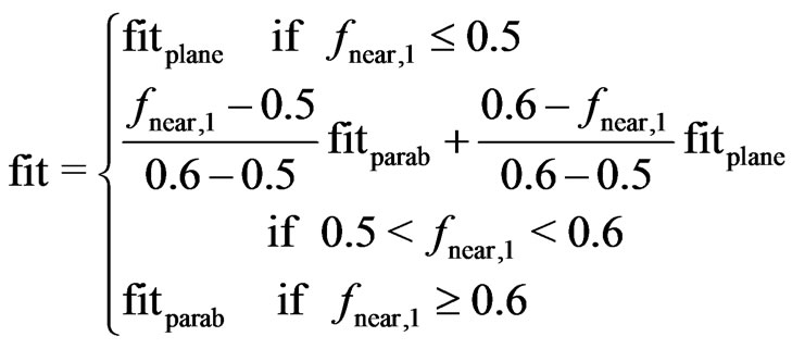 (29)
(29)
The measure , which it refers to, is based on the elliptical neighborhood with radii
 and
and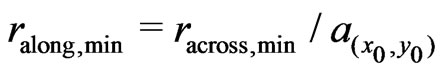 .
.
Modeling only a horizontal plane (p = 1) for very small  has proved inadequate because areas with only a few measurements occur mainly at corners of a field, where the yield usually tends to become lower. Instead, the neighborhood size is increased until
 ![]() reaches a minimum value of 0.30, so that there are enough data to fit an appropriate skewed plane.
reaches a minimum value of 0.30, so that there are enough data to fit an appropriate skewed plane.
2.5.5. Determining the Neighborhood’s Size
The neighborhood should also be enlarged if the effective number of data points, , is less than a minimum effective number,
 . This often applies where the combine enters the harvest track because the corresponding measurements have a global weight of zero. The rule for increasing the neighborhood's radii is as follows:
 (30)
(30)
The proportion,  , of
, of  to
to![]() , as well as the choice of model is no longer affected by this procedure, as these decisions have already been made on the basis of
, as well as the choice of model is no longer affected by this procedure, as these decisions have already been made on the basis of  and
and .
.
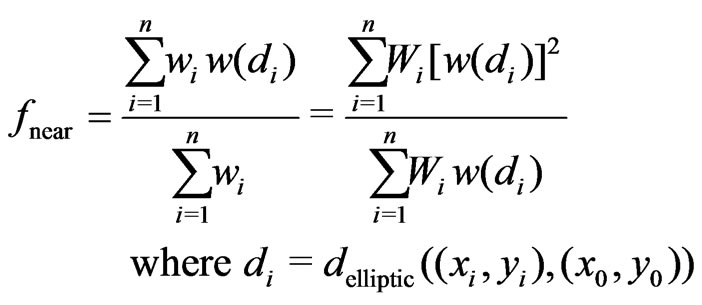
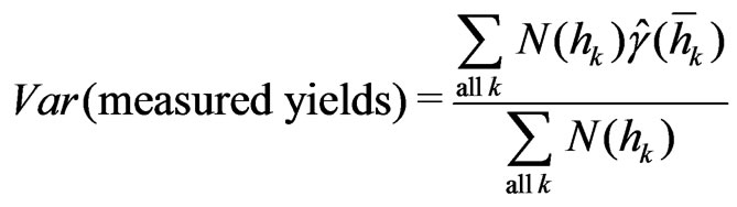
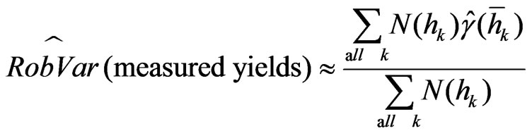
3. The Method of Finding an Adequate Neighborhood Size by Variance Comparison
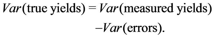
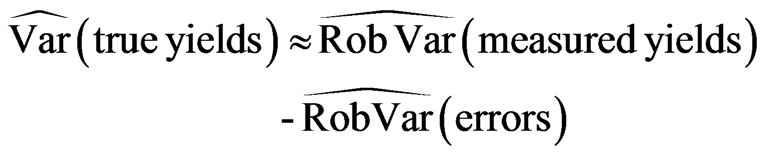
If the variance of the true unknown yields of the field were known, the yield map could be considered optimal if its variance equaled that of the true yields. If it is less than the variance of the true yields, the map is too smooth, if it is greater, the map is too detailed. The variance of the true yields is unknown. It needs to be estimated in a way that does not depend on how the yield map has been generated.
The variance of the measured yields comprises the variance of the true yields and the error variance of the yield monitor. Hence, the required variance of the true unknown yields results in
 (31)
(31)
The error variance,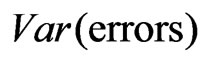 , can be estimated by the nugget component of a variogram. The reason is that there is no microscale variation in the yields because, as defined in the introduction, any yield at a field point refers to the average yield on a rectangle to be harvested around it, so all the nugget effect arising in an empirical variogram reduces to the error variance,
  , of the yield monitor (Cressie [16], p. 59). However, outliers often distort the structure of a variogram, which makes the determination of this value by extrapolation impossible unless outliers are removed or the variances are estimated robustly. Therefore, later I will switch to robust versions of variances and variograms. Nevertheless, for a better understanding it is desirable that the reader be familiar with the usual variogram, so I will introduce it first.
3.1. The Variogram
The empirical variance of measured values ![]() can be given by the following two equivalent formualae; the latter is less well known.
can be given by the following two equivalent formualae; the latter is less well known.
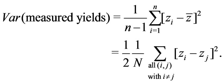 (32)
(32)
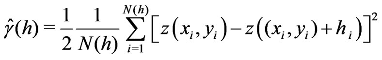
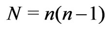 is the number of summands in the latter formula, which expresses the variance as half the average of the squared differences between all pairs of values. Squared differences of yields usually increase if the spatial distance between the data points increases. This is expressed by a variogram, which gives the variance as a function of the separation distance,
 , which is also called the lag. Empirical variances,
 , depicted in a variogram are restricted to pairs of values that are separated by a given lag
 , so they can be called variances of the yield data points at given separation distance
  (Bachmaier and Backes [17]):
 (33)
(33)
This writing is as usual as misleading. One must be aware that the index  in this sum is not a counter of certain logged locations (mean adjusted GPS points), but a counter of pairs of such locations. A single location can occur in many pairs, so that, for example, the third logged location point, which was denoted by
 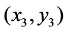 in Section 2, could now be indexed by
 . The index
  counts all pairs of those locations that are separated by a vector
 whose length,
![]() , is approximately equal to the target length
, is approximately equal to the target length , i.e.
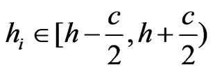 , where
 ![]() is the class width of distances used for computing a single variogram value (
is the class width of distances used for computing a single variogram value ( m in Figure 12).
  is the number of all these pairs.
The total variance of the measured yields in (32) is split into variances at given separation distance in (33), which in turn can be used to obtain the total variance as a weighted mean of them:
 (34)
(34)
where  correspond to the target distances
  in (33). They are the midpoints of the different classes, whereas
  are the averages of all distances within class
 , i.e.
the averages of all ![]() with
with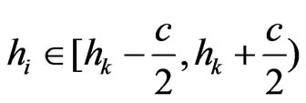 . An analogue of the formula in (34) is needed to compute the total variance robustly.
3.2. A Robust Variogram for Estimating the Variance of the True Yields
The variogram estimator  in (33) is based on squared differences among data, so it is sensitive to outlying yield data points. A single outlying datum can distort the variogram estimates since it occurs in several paired comparisons over many or all lag intervals (Lark [18]). Moreover, the outlier does not affect the variogram values of all lag intervals equally; it can distort the shape of the variogram, which affects the determination of the nugget component by extrapolation. Such distortion can be diminished by robust estimates of the variogram.
Robust variogram estimates have been introduced by several authors (Cressie and Hawkins [19], Dowd [20], Genton [21]). Lark [18] compared them with regard to robustness and efficiency. Since the formula of variance decomposition in (31) holds exactly only when referring to classical variances, I use a scale M-estimator whose  -function equals the classical one,
 , if
, if  where about 95% of standard normally distributed data are located. This guarantees a high efficiency for distributions close to normal (Bachmaier [22]). Outside the interval
  the chosen
  -function begins to deviate, and from
  it redescends until it reaches the value zero at
  to exclude the effect of large outliers completely. It is illustrated in Figure 9 and defined by parabolae and straight lines:
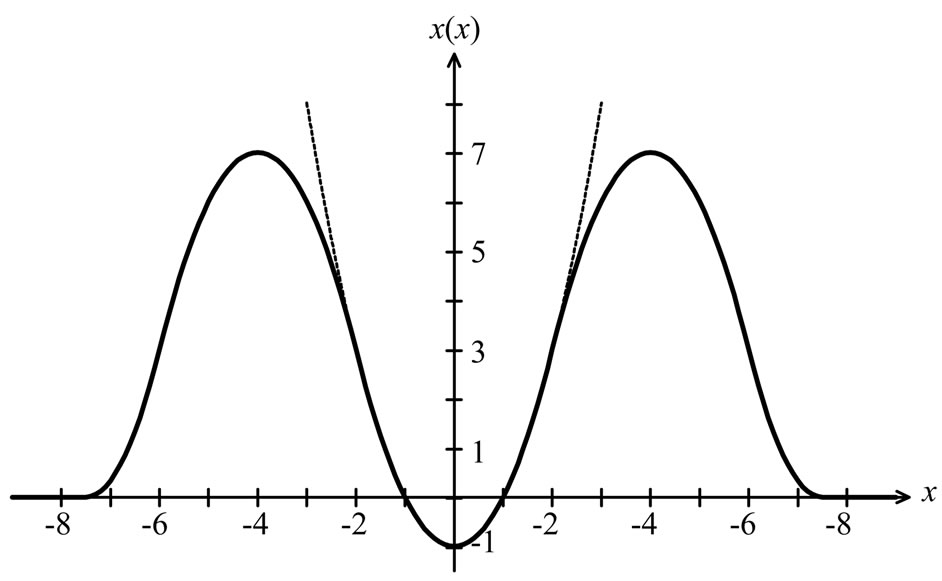
Figure 9. Redescending ![]() -function compared to the classical
-function compared to the classical ![]() -function.
-function.
 (35)
(35)
The robust variances, , at a target separation distance,
 , are then defined by the solution of
 (36)
(36)
with as in Figure 9, where the index
  again counts pairs. Note that the solution of (36) would correspond exactly to the classical variogram estimate
  in Eq. (33) if one replaced the
  -function in Figure 9 by the classical
  -function,
 .
.
To compute the robust variogram for the yield monitor data according to (36), it was necessary to omit summands related to pairs  that are close to each other on the same harvest track. This ensures near independence of the remaining pairs
 . Pairs where either
 ![]() or
or  has a global weight of zero were canceled also. Such a robust variogram is shown in Figure 12.
3.3. Estimating the Variance of the True Yields
The desired classical variance of the true unknown yields is now, analogous to (31), computed as the following difference of robust variances:
 (37)
(37)
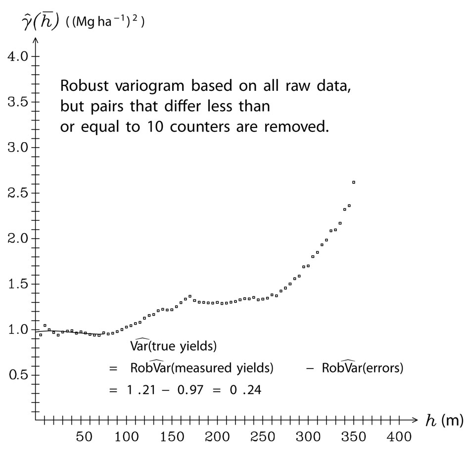
Figure 12. Robust variogram with the redescending ![]() -function in (35)
-function in (35)
The robust error variance at separation distance zero,
 (38)
(38)
which is the nugget component of the robust variogram, is determined by a weighted cubic extrapolation (Bachmaier [23]). The weights decrease linearly with increasing separation distance; in particular: ,
, ,
, , and
, and  for
for , where
  represents the class
 ,
,  the class
 , and so on.
Analogously to (34), the robust variance of all measured values, is estimated as a weighted mean of all values depicted in the robust variogram:
 . (39)
Thus, the variance estimation in (37) depends only on robust variogram values. They are barely affected by outliers, so they underestimate the theoretical classical variogram values a little, as these also include the variance of the yield monitor, which might be large because of the outliers. But since the underestimation of the robust variances affects all variances in the variogram similarly, the difference in (37), which gives the desired variance of the true yields, is barely affected. Therefore, this estimation method worked well, as shown in the Monte Carlo results in Bachmaier [23].
4. Results for the Field Bandstauden in Zeilitzheim
In 2001 the winter wheat harvest of Bandstauden field in Zeilitzheim (Germany) was investigated. Using the measurements for moisture, the raw yield data measured by the Claas Agrocom Quantimeter with a data logging frequency of 0.2 Hz were converted to dry matter yields. Zero yields were omitted as were those with a missing value for moisture. Values with technical errors were assigned the global weight zero, which meant they were discarded also.
Figures 10(a), (b) shows the yield monitor data in Mg ha-1 and their global weights, , respectively. Weights less than 1 arise from a small deviation from the preceding harvest path or from values at the beginning of a swath. Many neighboring swathes were harvested in the same direction, therefore, regions with invalid values are larger than usual.
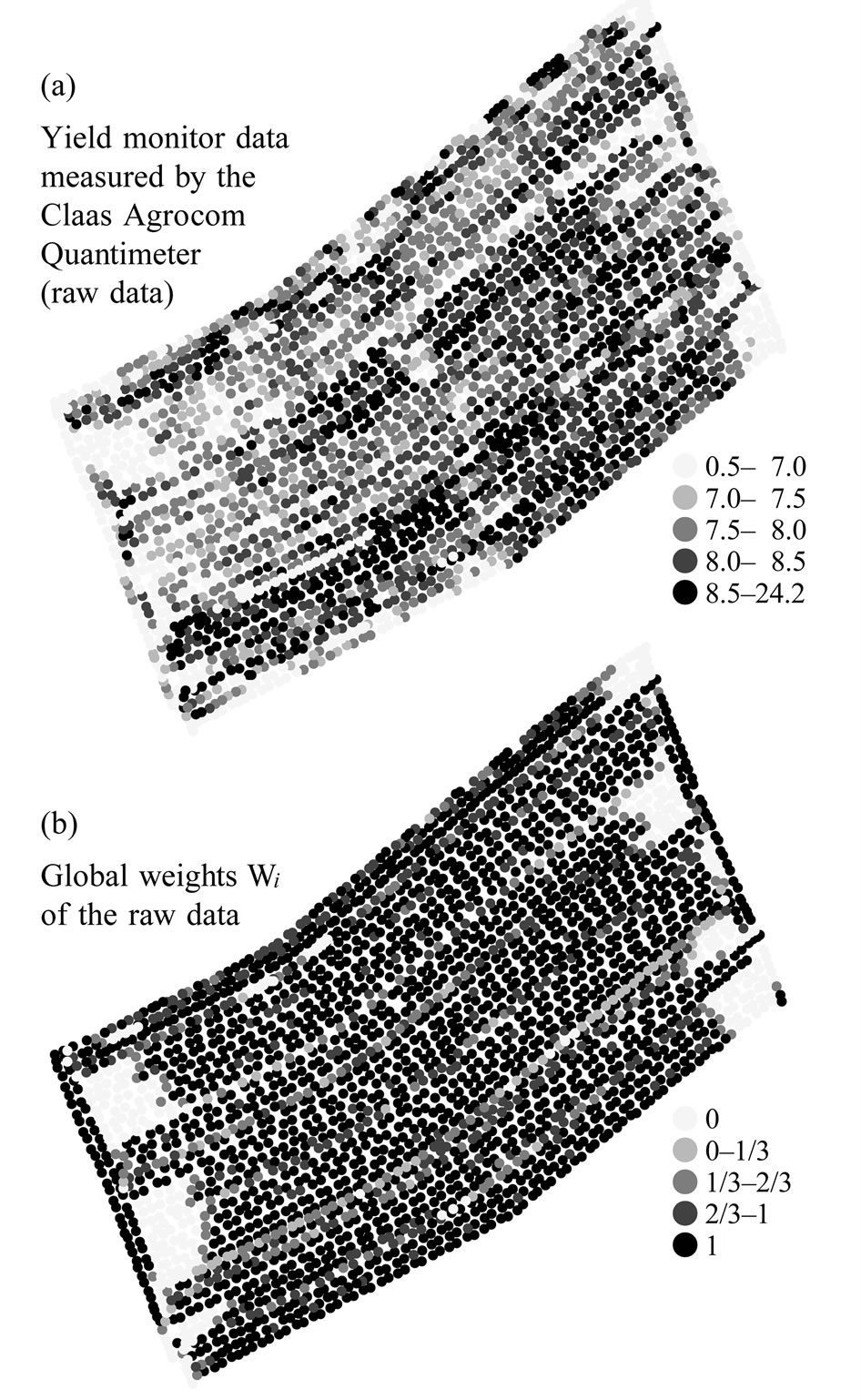
Figure 10. Raw data ![]() in Mg ha-1 and their global weights
in Mg ha-1 and their global weights 
4.1. Yield Maps Generated Using Different Neighborhood Size
Figure 11 shows three yield maps for different sizes of an elliptical neighborhood with a radius ratio of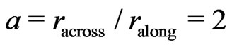 . It decreases according to
  in (28) if a point is mapped whose nearer environment does not contain enough valid data points.
The larger the neighborhood size, the smoother the yield map is and the less is its variance. With a fine -textured yield map in Figure 11(a), there is a risk that it shows the errors of the yield monitor too clearly, whereas Figure 11(c) shows too much smoothing. To determine approximate degree of smoothness of the yield map, the variance of the true unknown yields must be obtained and compared with the variances given in Figure 11.
4.2. The Adequate Smoothness of the Yield Map
An adequate neighborhood size is obtained if the variance of the yield map equals that of the true yields. The variance estimation of the true yields is described from (36) to (39). It is based on the robust variogram in Figure 12, which clearly contains a trend component of the unknown yield map. Note that such a variogram would not be appropriate to determine kriging weights. For this, the variogram should be trend-adjusted. But a variogram that serves to determine the variance of the yield map must also contain the trend, as the trend is an essential part of it. The robust variogram in Figure 12 is drawn at the points , the mean of values
 ![]() within class
within class .
.
According to (37), the variance of the true yields is estimated by
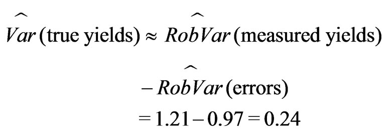 (40)
(40)
where the robust error variance, 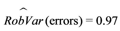 , equals the nugget component,
  , which was obtained as the intercept on the ordinate of the extrapolated robust variogram in Figure 12. The robust variance of all measured values,
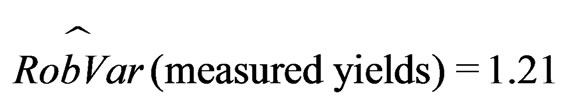 , was computed as the weighted mean in (39), which refers to all values depicted in the robust variogram.
Since the yield map is required to be as smooth as the true yields, Figure 11(b) should be chosen because its variance of 0.242 equals the estimated variance of the true unknown yields in (40). The elliptical neighborhood used to generate this yield map started with a minimum  of ten times the swath width (and, since
 ,
,
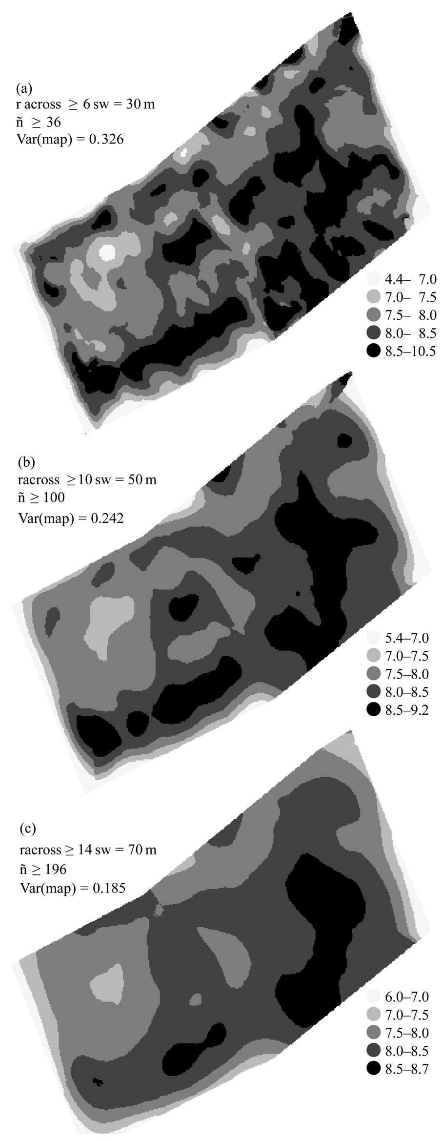
Figure 11. Yield maps (in Mg ha-1) for different sizes of an elliptical neighborhood with 
with a minimum ![]() of five times the swath width) and was increased until the minimum effective number of data reached
of five times the swath width) and was increased until the minimum effective number of data reached . This number needs to be adapted to the neighborhood size. It should approximately correspond to the that
 ![]() which is expected if most measurements of the neighborhood are valid. It depends on the data logging frequency, on the swath width, and, of course, on the neighborhood size.
which is expected if most measurements of the neighborhood are valid. It depends on the data logging frequency, on the swath width, and, of course, on the neighborhood size.
5. Discussion and Conclusions
The yield mapping method proposed in this article is based mainly on modeling paraboloid cones on moving elliptical neighborhoods. The method of determining the parameters of the model is robust, so that the detection of outliers was not necessary. Besides, the method refers to weights that decrease, like a paraboloid cone opening downwards, to zero at the neighborhood’s border. This corresponds to a smooth transition from being fully considered to being not considered at all, so that a larger neighborhood is necessary, as the values close to the border do not have full weight. A robust variogram, computed independently of the yield mapping method, served to estimate the variance of the true unknown yield values. This provided a measure of how smooth the yield map would be if all values had been measured correctly. For an elliptical neighborhood with at least ,
,  (i.e.
(i.e. ) and a minimum effective number of
  the estimated yield map had the same variance as the true unknown yield map.
In 2004, an experiment was done on a part of the Lamprechtsfeld in Thalhausen (Germany) where measured reference values for yield data from two yield monitors were obtained; Data Vision Flowcontrol and AgLeader. The results based on butterfly neighborhoods suggest that, if one wants a yield map whose sum of squared deviations from the true unknown values is minimized, the neighborhood size should be greater than that of Figure 11(b). However, the yield map optimized under this criterion is much smoother than the map of the true reference values, i.e., its variance is too small. In Bachmaier et al. [24], where these results are published, the shape of the butterfly neighborhood was also optimized.
The method proposed in the present paper cannot be used to optimize the neighborhood’s shape, but it gets along with yield monitor data only. It could already be seen from Figure 9(a). in Bachmaier [1] that a circular neighborhood did not sufficiently smooth out the yield data across the tracks; these or other lines cannot be recognized in the present Figure 11, which is based on an elliptical neighborhood that is twice as long ( ) across the tracks than it is along them. Therefore, a radius ratio of
  might be a good choice.
Currently, the proposed method is applied to a single yield monitor only (Claas Agrocom Quantimeter) with a data logging frequency of 0.2 Hz and one crop. It could also be applied to harvests from other crops or from combines equipped with other cutting widths and other yield monitors. This might lead to different results, however, the yield mapping rule proposed here would produce yield maps that are not too smooth, not too fine-textured and not subject to large outliers. The reason is that it requires at least a radius of  and it does not depend on the swath width, sw, because the radii are expressed in multiples of it. This also guarantees robustness against exclusively erroneous measurements on one or two harvest tracks within the neighborhood. The method requires a minimum effective number of data,
 . A yield monitor with a higher frequency, such as the AgLeader monitor, provides more data, so
  would be reached within a smaller neighborhood. But these data are usually less accurate, so the neighborhood size should not decrease. What should be adapted to the yield monitor is the number,
![]() ,of zero -weights at the beginning of harvest tracks. It should increase with the frequency of the system and be adapted to the intensity of its smoothing algorithm. In the Fortran program paraboloidmapping (Bachmaier [25]), where the yield mapping method is implemented, I currently use m = 5 for Claas Agrocom,
,of zero -weights at the beginning of harvest tracks. It should increase with the frequency of the system and be adapted to the intensity of its smoothing algorithm. In the Fortran program paraboloidmapping (Bachmaier [25]), where the yield mapping method is implemented, I currently use m = 5 for Claas Agrocom,  for Data Vision Flowcontrol, which has a stronger smoothing algorithm, and
  for AgLeader because of its high frequency of 1 Hz.
6. Acknowledgements
I thank Margaret A. Oliver, University of Reading, for her helpful and detailed remarks on this research and Hermann Auernhammer, Technische Universität München-Weihenstephan, for supporting this work.
REFERENCES
- M. Bachmaier, “Using a Robust Variogram to Find an Adequate Butterfly Neighborhood Size for One-Step Yield Mapping Using Robust Fitting Paraboloid Cones,” Precision Agriculture, Vol. 8, No. 1-2, 2007, pp. 75-93.
- G. C. Simbahan, A. Dobermann and J. L. Ping, “SiteSpecific Management.Screening Yield Monitor Data Improves Grain Yield Maps,” Agronomy Journal, Vol. 96, 2004, pp. 1091-1102.
- S. A. Shearer, S. G. Higgins, S. G. McNeil, G. A. Watkins, R. I. Barnhisel, J. C. Doyle, J. H. Leach and J. P. Fulton, “Data Filtering and Correction Techniques for Generating Yield Maps from Multiple Combine Harvesting Systems,” ASAE Paper No. 971034, Annual International Meeting, Minneapolis Minnesota, 10-14 August 1997.
- B. S. Blackmore and M. Moore, “Remedial Correction of Yield Map Data,” Precision Agriculture, Vol. 1, No. 1, 1999, pp. 53-66.
- S. Arslan and T. S. Colvin, “Grain Yield Mapping: Yield Sensing, Yield Reconstruction, and Errors,” Precision Agriculture, Vol. 3, No. 2, 2002, pp. 135-154.
- T. Steinmayr, “Fehleranalyse und Fehlerkorrektur bei der lokalen Ertragsermittlung im Mähdrescher zur Ableitung eines standardisierten Algorithmus für die Ertragskartierung,” Dissertation at the Technische Universität München-Weihenstephan, 2003, pp. 24-27.
- L. Thylén, P. A. Algerbo and A. Giebel, “An Expert Filter Removing Erroneous Yield Data,” In: Robert et al., Ed., Precision Agriculture 2000: Proceedings of the 5th International Conference on Precision Agriculture, ASA, CSSA, and SSSA, Madison, WI, CD-ROM, 2001.
- L. Thylén, P. Jürschik and D. P. L. Murphy, “Improving the Quality of Yield Data,” In: J. V. Stafford, Ed., Precision Agriculture '97: Proceedings of the 1st European Conference on Precision Agriculture, BIOS Scientific Publishers Ltd, Oxford, UK, 1997, pp. 743-750.
- P. H .Noack, T. Muhr and M. Demmel, “An Algorithm for Automatic Detection and Elimination of Defective Yield Data,” In: J.V. Stafford and A. Werner, Ed., Precision Agriculture, Wageninen Academic Publishers, Wageningen, 2003, pp. 445-450.
- F. R. Hampel, P. J. Rousseeuw, E. M. Ronchetti and W. A. Stahel, “Robust Statistics,” John Wiley & Sons, Inc., New York, USA, 1986.
- M. Bachmaier and H. Auernhammer, “Yield Mapping Based on Robust Fitting Paraboloid Cones in Butterfly and Elliptic Neighborhoods,” In: J. V. Stafford and A. Werner, Ed., Precision Agriculture '05: Proceedings of the 5th European Conference on Precision Agriculture, Wageningen Academic Publishers, Wageningen, the Netherlands, 2005, pp. 741-750.
- P. J. Huber, “Robust Statistics,” John Wiley & Sons, Inc., New York, USA, 1981.
- F. W. Satterthwaite, “An Approximate Distribution of Estimates of Variance Components,” Biometrics Bulletin, Vol. 2, No. 6, 1946, pp. 110-114.
- P. J. Huber, “Robust Statistical Procedures,” Regional Conference Series in Applied Mathematics 27, Society for Industrial and Applied Mathematics, Philadelphia, Pennsylvania, 1977.
- M. Bachmaier and H. Auernhammer, “A Method for Correcting Raw Yield Data by Fitting Paraboloid Cones,” In: Proceedings of the AgEng 2004 Conference — Engineering the Future, Session 10: Precision Agriculture, 8 pages on CD-ROM, 2004.
- N. A. C. Cressie, “Statistics for Spatial Data,” John Wiley & Sons, Inc., New York, USA, 1991.
- M. Bachmaier and M.Backes, “Variogram or Semivariogram? — Understanding the Variances in a Variogram,” Precision Agriculture, Vol. 9, No. 3, 2008, pp. 173-175.
- R. M. Lark, “A Comparison of Some Robust Estimators of the Variogram for Use in Soil Survey,” European Journal of Soil Science, Vol. 51, No. 1, 2000, pp. 137-157.
- N. A. C. Cressie and D. Hawkins, “Robust Estimation of the Variogram,” Mathematical Geology, Vol. 12, No. 2, 1980, pp. 115-125.
- P. A. Dowd, “The Variogram and Kriging: Robust and Resistant Estimators,” In: G. Verly et al., Ed., Geostatistics for Natural Resources Characterization, D. Reidel, Dordrecht, Part 1, 1984, pp. 91-106.
- M. G. Genton, “Highly Robust Variogram Estimation,” Mathematical Geology, Vol. 30, No. 2, 1998, pp. 213-221.
- M. Bachmaier, “Efficiency Comparison of M-Estimates for Scale at T-Distributions,” Statistical Papers, Vol. 41, 2000, pp. 53-64.
- M. Bachmaier, “Finding Adequate Neighborhoods for Robust Yield Mapping,” 2006. http://www.tec.wzw.tum. de/ index.php?id=46
- M. Bachmaier, M. Rothmund and H.Auernhammer, An “Attempt to Optimize Yield Maps by Comparing Yield Data from a Plot Combine and from a Combine Harvester,” Agricultural Engineering International, Manuscript IT 07 009, Vol. 10, 12 pages, 2008. http://cigrejournal.tamu.edu
- M. Bachmaier, Fortran-Programme zum Herunterladen: Korrektur von Rohertragsdaten und Ertragskartierung: DOS/Windows-Programme paraboloidmapping.exe, 2010.
- und paraboloidcorrection.exe (in English). http://www.tec. wzw.tum.de/index.php?id=46