Engineering
Vol.08 No.09(2016), Article ID:70590,21 pages
10.4236/eng.2016.89055
Phoneme Sequence Modeling in the Context of Speech Signal Recognition in Language “Baoule”
Hyacinthe Konan1*, Etienne Soro1, Olivier Asseu1,2*, Bi Tra Goore2, Raymond Gbegbe2
1Ecole Supérieure Africaine des Technologies d’Information et de Communication (ESATIC), Abidjan, Côte d’Ivoire
2Institut National Polytechnique Félix Houphouët Boigny (INP-HB), Yamoussoukro, Côte d’Ivoire

Copyright © 2016 by authors and Scientific Research Publishing Inc.
This work is licensed under the Creative Commons Attribution International License (CC BY 4.0).
http://creativecommons.org/licenses/by/4.0/


Received: August 9, 2016; Accepted: September 10, 2016; Published: September 14, 2016
ABSTRACT
This paper presents the recognition of “Baoule” spoken sentences, a language of Côte d’Ivoire. Several formalisms allow the modelling of an automatic speech recognition system. The one we used to realize our system is based on Hidden Markov Models (HMM) discreet. Our goal in this article is to present a system for the recognition of the Baoule word. We present three classical problems and develop different algorithms able to resolve them. We then execute these algorithms with concrete examples.
Keywords:
HMM, MATLAB, Language Model, Acoustic Model, Recognition Automatic Speech

1. Introduction
The speech recognition by machine has long been a research topic that fascinates the public and remains a challenge for specialists, and it has continued since then to be at the heart of much research. The progress of new information and communications technology has helped accelerate this research. In our first article, we presented a method to separate phonemes contained in a speech signal.
In this article we propose to identify a flow of words often uttered in a more or less background noise. This task is made difficult not only by the deformations induced by the use of a microphone but also by a series of factors inherent in human language, homonyms; local accents; the habits of language; the speed differences between the speakers; the imperfections of a microphone, etc. For our human ear, these factors do not usually represent difficulties. Our brain juggles these deformations of speech by taking into account, almost unconsciously, nonverbal and contextual elements that allow us to eliminate ambiguities. It is only by taking into account these elements that are external to the voice itself that voice recognition software will be able to achieve a high level of reliability. Today, speech recognition softwares that work best are all based on a probabilistic approach. The aim of speech recognition is to reconstruct a sequence of words M from a recorded acoustic signal A. In the statistical approach, we will consider all the consequences of M words that could match the signal A. In this set of possible word sequences, we will then choose the one (M) which is the most likely to maximize the P(M/A) probability that M is the correct interpretation of A, we note:
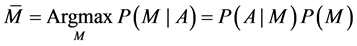
This equation is the key to the probabilistic approach to speech recognition. Indeed, the first term P(A/M) is the probability of observing the acoustic signal A if the M sequence of words is pronounced: it is a purely acoustic problem; the second term P(M) is the probability that this is the result of M words that is actually stated: it is a linguistic problem. The above equation thus teaches us that we can split the speech recognition problem into two independent parts: we will model the acoustic aspects separately and language problems. In the literature, we usually speak of orthogonality between the ACOUSTIC MODELS and LANGUAGE. The succession of possible words that is obtained must be refined and validated by the word patterns and language. The acoustic model can take into account the acoustic and phonetic constraints in a sound or group of sounds. On our part, we have chosen the WORD as decision unit. By integrating also a Markov modeling, which has higher levels of language, it becomes possible to achieve a pronounced phrases discretely recognition system (i.e. in single word).
2. The Speech Signals
2.1. Characteristics of the Speech Signal
PAR is a difficult problem, mainly due to the specific material to interpret: the voice signal. The speech acoustic signal has characteristics that make complex interpretation.
Redundancy: the acoustic signal carries much more information than necessary, which explains its resistance to noise. Of analytical techniques were implemented to extract relevant information without too degrading it.
Variability: the acoustic signal is highly variable from one speaker to the other (gender, age, etc.) but also for a given speaker (emotional state, fatigue, etc.), which makes very difficult the recognition problem speaker’s independent speech.
Continuity: the acoustic signal is continuous and contextual effects of sound on elementary visions are considerable.
2.2. Processing of the Speech Signal
By speech processing we mean the processing of the information contained in the speech signal. The objective is the transmission or recording of this signal, or its synthesis or recognition. The speech processing is now a fundamental component of the engineering sciences. Located at the intersection of digital signal processing and language processing (that is to say, symbolic data processing), this scientific discipline has known since the 60s a rapid expansion, linked to the development of means and telecommunications techniques. The special importance of speech processing in this broader context is explained by the privileged position of the word as an information vector in our human society.
3. System Overview
3.1. The Acoustic Model
The ACOUSTIC MODEL (Figure 1) reflects the acoustic realization of each modeled element (phoneme, silence, noise, etc.). It is based on the concept of phonemes. Phonemes can be considered as the basic sound units in verbal language. The first stage of speech recognition is to recognize a set of phonemes in words flow. Statistical realization of acoustic parameters of each phone is represented by a Markov model Cache (HMM: Hidden Markov Model). Each phoneme is typically represented by 2 or 3 states and density multigaussienne (GMM: Gaussian Mixture Model) is associated with each state. See Figure 2 below.
The speech signal (picked up using a microphone) is first digitized: it is sampled by a Fourier transformation which calculates the energy levels of the signal in bands of 25 milliseconds, which strips overlap in 10 milliseconds time.
The result is compared with prototypes stored in computer memory in both a standard dictionary and a speaker’s own dictionary. This dictionary is constructed by initially sessions dictation standard texts that the speaker must make before effectively use the software. This own dictionary is regularly enriched by self learning during the software uses. It is interesting to note that thus constituted voiceprint is relatively stable for a given speaker and little influenced by external factors such as stress, colds, etc. (Figure 3).
3.2. The Language Model
It is generally divided into two part linked to language: a syntactic part and a semantic game. When ACOUSTIC MODEL has identified at best phonemes “heard”, we still look the most likely message M corresponding thereto, that is to say, the probability P(M) defined above. It is the role of syntactic and semantic models. See Figure 4 below.
From the set of phonemes from the ACOUSTIC MODEL The SYNTACTIC MODEL will assemble phonemes into words. This work is also based on a dictionary and gram-

Figure 1. System of speech recognition.

Figure 2. The part of the system using the acoustic model.


Figure 3. Acoustic model (A phoneme is modeled as a sequence of acoustic vector).

Figure 4. The part of the system using the semantic model.
mar standards (The language “Baoule” has one) as well as a dictionary and a grammar own speaker; these reflect the “habits” of the speaker and is continuously enriched. Then SEMANTIC MODEL seeks to optimize the identification of the message by analyzing the context of the words and while basing on both its own common language semantics and on cleanning the speaker semantics (a style). This modeling is usually built from the analysis of sequences of words from a large textual corpus. This clean semantics will be enriched as you use the software. Most softwares also allow enriching the analysis of texts that reflect the stylistic habits of the speaker. These two modules work together and it is easy to conceive that there is a feedback between them.
Initially, the dictionary associated with these two modules were based on fixed syntax language models, that is to say, modeled on a grammar defined by a rigid set of rules (this is not the case in most African languages including the “Baoule” language).
Then, the voice recognition software has evolved into the use of local probabilistic models: recognition no longer performs at a word but at a series of words, called n-gram where n is the length words in a sequence .The statistics of these models are obtained from standard texts and may be enriched gradually. See Figure 5 below.
Here too, Hidden Markov Models are those currently used to describe the probabilistic aspects. the most advanced software tend to combine the advantages of statistical models and fixed syntax models in what is called the “probabilistic grammars”, the idea being to derive from fixed grammars of probabilities that can be combined with those of a probabilistic model. In recent approaches, it becomes difficult to distinguish the syntactic model of the semantic model and we rather speak of a single language model.
4. Hidden Markov Model Discrete Time
4.1. Overview and Features
4.1.1. Fundamentals
Hidden Markov Models (HMM) were introduced by Baum and his collaborators in the 60s and the 70s [1] . This model is closely related to Probabilistic Automata (PAs) [2] . A probabilistic automaton is defined by a structure composed of states and transitions, and a set of probability distribution on transitions. Each transition is associated with a symbol of a finite alphabet. This symbol is generated every time the transition is taken. An HMM is also defined by a structure consisting of states and transitions and by

Figure 5. Semantic model.
a set of probability distribution over the transitions. The essential difference is that the IPs symbol generation is performed on the states, and not on transitions. In addition, is associated with each symbol, not a state, but a probability distribution of the symbols of the alphabet.
HMMs are used to model the observation sequences. These observations may be discrete (e.g., characters from a finite alphabet) or continuous (the frequency of a signal, a temperature, etc.). The first area in which the HMMs have been applied is the speech processing in early 1970 [3] [4] . In this area, the HMM will rapidly become the reference model, and most of the techniques for using and implementing HMM have been developed in the context of these applications. These techniques were then applied and adapted successfully to the problem of recognition of handwritten texts [5] [6] and analysis of biological sequences [7] [8] . Theorems, rating and proposals that follow are largely from [9] .
4.1.2. Characteristics of HMM
A sequence  of random variables with values in a finite set E is a Markov chain if the following property holds (Markov property):
 for any time k and any suite
Note that notion generalizes the notion of deterministic dynamical system (finite state machine recurrent sequence, or ordinary differential equation): the probability distribution of the present state  depends only on the immediate past state
 .
.
A Markov chain  is entirely characterized by the data
・ the original legislation ;
;  for all
・ and the transition matrix ;
;  for all
supposedly independent of time k (homogeneous Markov chain).
Knowing the transition probabilities that exist between two succesive times is enough to globally characterize a Markov chain.
Proposal
 is a probability on E, and
  a Markov matrix E
The probability distribution of the Markov chain  of
of  original legislation and
  transition matrix is given by
 for any time k, and any suite
In this model the suite is not observed directly after , but observations are available
  with values in a finite space O (if symbolic) or
  (digital case), collected through a channel without memory, that is to say, conditionally to
  states.
i. the observations  are mutually independent, and
ii. each observation  depends only on the
  at the same time
This property is expressed as follows:
 for any result,
  , and every sequence
Example
Assume that the observations  are connected with states
  follows
  where the sequence
  is a Gaussian white noise dimension, with zero mean and covariance matrix R reversible, independent of the Markov chain
  function h defined on E with values in
  is characterized by the data of a finite family
  vectors of
 , and was

conditionally to , random vectors
  are mutually independent, and each
  is a Gaussian random vector of dimension d, medium
  and R covariance matrix so that no memory channel property is verified.
A hidden Markov model  is fully characterized by the particular
The original legislation ;
;  for all
The transition matrix ;
;  for all
  andemission densities
 ;
;  for all
  for any and all
 .
.
So just a local data (transition probabilities between two successive times, and densities of issue at a time) comprehensively characterizes a hidden Markov model, example: for K = 3, it comes:

Proposal: The probability distribution of the hidden Markov model  initial
  law of
  transition matrix, and g emission densities, is given by
for all time k following , and every sequence
  is denoted by
 , the parameters characteristic of the model, and we focus on three issues:
Problem No. 1: Evaluate the model: it comes to efficiently compute the probability distribution of the following observations  (or likelihood function) according to the parameters of the model M. The answer to this problem is provided by the forward Baum equation.
Problem No. 2: Identify the model: given a series of observations , this is to calculate the maximum likelihood estimator for the unknown parameters of the model M. The answer to this problem is provided by the re-estimation formulas of Baum-Welch, defining an iterative algorithm to maximize the likelihood function.
Problem No. 3: Estimate the condition of the system: given a sequence of obser- vations , it is to estimated recursively the state
  (filtering Song), or a good estimate
  intermediate state for
  (smoothing Song), or an overall estimate of the sequence of states
 , for a given model M. the response to first two problems is provided by the forward and backward equations Baum, which calculate the conditional probability distribution of
  state given observations
 .
.
The answer to the last problem is provided by a dynamic programming algorithm, the Viterbi algorithm, which maximizes the conditional probability distribution of the sequence of states  given observations
 .
.
4.2. Equations Forward/Backward Baum
We first present a first method (basic but inefficient) to calculate the probability dis- tribution of observations .
.
Proposal: The probability distribution of observations  is given (in the digital case) by
 for any sequence
 .
.
Note that elementary method provides a first expression for the conditional probabi- lity distribution of the sequence of states  given observations
  (in digital case):

and the likelihood of the model (obtained using the following observations  in place of dummy variables):

we deduce the following identities:
 .
.
Note the number of operations required to calculate the probability distribution of observations  from this basic method is significant for each possible path
  of the Markov chain, you must compute the product of
  words, and there is
  different possible paths the total number of elementary operations (additions and multiplications) thus made is of the order of
  the number is growing exponentially with the number n of observations. we define the forward
  (seen as a row vector) by
  for all
 .
.
Note the forward variable used to calculate the conditional probability distribution of
the present state  given observations
 :
: 
for all . (In this sense,
  is a distribution of non-normalized probability), and the normalization constant
  is interpreted as the likelihood of the model given observations
 .
.
Theorem: The sequence  satisfies the following recurrence equation:
 for all
  with the initial condition
  for any
 .
.
Note this statement result component-by-component can also be made for the variable forward view as a row vector  and
and .
.
Note the recursive calculation of the variable forward  involves only the product matrix/vector, and to calculate more efficiently the probability distribution of obser- vations
  simply
  elementary operations (additions and multi- plications) to move from time k to time
  the total number of elementary operations to be performed is thus of the order of:
  this number grows only linearly with the number n of observations.
Digital implementation: Instead of first solving the equation for the forward non-standardized version of the conditional distribution, defined at any time k as  for all
  and then deduct the normalization constant (likelihood) and the normalized version of the conditional distribution (filter)
 and
and 
It is more efficient, on a digital point of view, spread directly log-likelihood and filter.
Proposal: Following  Verie the following recurrent equation:
 for all
  with the initial condition
 for any
 .
.
where the normalization constants are defined by  and
and .
.
Note this result statement component-by-component may also be formulated for the
normalized forward variable seen as a row vector  and
and 
where the normalization constants are defined by  and
and .
.
Note: Following  truth the following recurrent equation:
 with the initial condition
  and iterating log
 . For all intermediate time k, less than the final instant n, is defined
  for all
 .
.
Note: That variable allows to calculate the conditional probability distribution of the
present state  knowing all comments
 ,
, 
for all  with the normalization constant
 .
.
Note: Fix the state at time k allows a break between the past up to time  and the future from time
 . This justifies the introduction of the variable backward
  (seen as a column vector) and defined as:
 for any
and in particular  for all
  with this definition, is obtained
  for all
 .
.
Note: Conditionally  the X_ suite
  to come hidden states is a Markov chain, from initial law
  (line i the
  matrix), that is to say that
  for all
  and
and  transition matrix it follows that the backward variable can be interpreted as the likelihood of the model derived from the
  state at time k given observations
 .
.
Theorem:
After  Verie recurrent retrograde following equation:
 for all
  with the initial condition:
  for all
 .
.
Note: This result statement component-by-component can also be formulated for the backward view variable as a column vector  and
and .
.
Proposal: the forward and backward equations are dual to one another:
 not dependent of the time in question
Proposal: For the distribution of conditional probability of transition  at an intermediate time given observations
  until the final moment is given by:
 for all
By summing for all  and using the equation backward, or by summing for all i ∈ E and using the forward equation, we find the following results in terms of product component-by-component variables forward and backward.
Corollary: the conditional probability distribution of the present state  knowing
all comments  is given by
  with the definition
 for all
 .
.
Note: Verie one that constant Standards

and 
do not depend on the time in question, and are interpreted as the likelihood of the model given observations . instead of first solve the backward and forward equation equation separately, and to successively deduct the non-normalized version of the conditional distribution, defined at any instant k as
  for all
then the normalized version of the conditional distribution (smoother)
 .
.
It is more efficient on a digital point of view, spread directly log-likelihood and filter,
then spread the variable defned at any time k as  for any
 .
.
Note: That with normalization of the backward variable, the conditional probability distribution of  state given observations
  is expressed as
 for all
 .
.
Proposal: Following  Verie recurrent retrograde following equation:
 for all
 , with the initial condition:
  for all
 where the normalization constants are those already defined for the normali- zation of the variable forward.
Note: This result statement component-by-component can also be formulated for
backward standardized variable viewed as a column vector  and
and
 where the normalization constants are those already defined for the normalization of the variable forward.
Note: It is noted that  for all
And postponing this identity in the expressions obtained above, we Verie that the conditional probability distribution of the transition  given observations
  is expressed as
 for
for .
.
4.3. Viterbi Algorithm
Forward and backward variables used to calculate the conditional probability distribution of the state this , or
, or  state at an intermediate moment, given observations
 defined by
  for all
 , and
, and
 for any
  respectively, where the normalization con-
stant  does not depend on the time in question, and interprets as the likelihood of the model given observations
 . it is not necessary to calculate the conditional average, but can be used however the estimator of maximum a posteriori, which minimizes the likelihood of the estimation error given observations
  and defined for the present state
 and for the state to an inter-
mediate time by  it may hap-
pen that the sequence  generated is inconsistent with the model, in the following sense: it can happen that is obtained
  and
and  for two successive times, while
  for the same pair
 , which meant that the transition from state i to state j is just impossible for the model for this reason, rather it uses another estimator, called trajectoriel maximum a posteriori estimator, defined by
 .
.
And minimizes the probability of the estimation error of the sequence of hidden states given observations  it is of course not possible to perform this maximization exhaustive manner, listing all
  possible trajectories: the efficient calculation of this estimator is provided by a dynamic programming algorithm called Viterbi algorithm.
4.4. Re-Estimation Formulas Baum-Welch
So far, the focus was on the estimation of a hidden condition or because of successive hidden states, from a series of observations and for a given model. The goal here is to identifier the model, that is to say, to estimate the parameters of the model characteristics, from a series of observations, and the approach taken is that of estimation maximum likelihood.
In the digital case, we look at the case of the Gaussian emission densities characterized by the data of finite 
 vectors and of finite Family
  matrices invertible covariance, that is to say:

The likelihood function of the model  admits expression

obtained with the basic method, and we will study an iterative algorithm to maximize  likelihood function with respect to the parameters
  model of either
  another model, for which the likelihood function takes the value

the (log) likelihood ratio between the  and the
  is reduced by

which vanishes when the model  coincides with the model
 .
.
Maximize  compared with parameters
  of the model
  thus ensures that the likelihood of the model which achieved maximum
  will be greater than the likelihood
  current model
  re-formulas Baum-Welch -Estimated allow explicitly find the parameters of the new model based on parameters
  of the current model
  by repeating this procedure, we construct a sequence of increasing likelihood models, and ideally this sequence converges to a model that reaches the maximum likelihood function.
Theorem
In the digital case with densities of Gaussian issue, the iterative algorithm for esti- mating the maximum likelihood of the model parameters from the observations , is given by explicit formulas re-estimate
 and
and  and
and
 and
and 
for all  where the two sequences
  and
and  are the standard equations of forward and backward solutions respectively for values
  parameters.
Note: Concretely, if  denotes the current model in step
  of the algorithm, then for values
  the para- meters are calculated standardized solutions
  and
and  of equations forward and backward respectively the parameters
  is calculated using the formulas to re-estimate what defines the new model
  to s next step of the algorithm.
5. Implementation
Our model is based on acoustic signal parameters. These parameters are obtained by calculating cepstral coefficients according to a Mel scale (MFCC Mel Frequency Cepstral Coefficients). Statistical realization of acoustic parameters of each phoneme is represented by a Hidden Markov model. Each phoneme is typically represented by 2 or 3 states, and multigaussienne density (GMM: Gaussian Mixture Model) is associated with each state. GMM densities with a large number of components designed to address multiple sources of variability that are affecting the speech signals (sex and age of the speaker, accent, noise).
For example: With the following data: Number of States (K = 2); π = [0.95 0.05; 0.05 0.95]; h = [−1 1]; σ2 = [3 3]; υ = [0.5 0.5]; we have the Figure 6 below.
A robust speech recognition system combines accuracy of identification with the ability to filter noise and adapt to other acoustical conditions such as speech and emphasis of the speaker. The design of a robust speech recognition algorithm is a complex task which requires detailed knowledge of signal processing and statistical modeling. Most speech recognition systems are classified as isolated or continuous. The isolated

Figure 6. Graphic representation of the Hidden Markov Model.
word recognition requires a short pause between each spoken word, while the speech recognition does not continue. Speech recognition systems can be classified as a dependent or speaker-independent. Speaker dependent system recognizes only the word of the voice of a particular speaker, while an independent speaker system can recognize any voice.
The implementation presented here uses features integrated into MATLAB and related products to develop the recognition algorithm. There are two main steps in the recognition of isolated words:
・ a learning phase and
・ a test phase.
The learning phase teaches the system by building its dictionary, an acoustic model for each word that the system has to recognize. In our example, the dictionary includes the numbers “zero” to “nine” in “Baoule” language. The test phase uses acoustic models of these numbers to recognize isolated words using a classification algorithm. We start with the the speech signal acquisition, and then we end with its analysis.
5.1. Speech Signal Acquisition
During the learning phase, it is necessary to record the repeated statements of each digit in the dictionary. For example, we repeat the word “nnou” (which means five in “Baoule” language) many times with a pause between each statement. That word will be saved in the file 'cinq.wav'. Using the following MATLAB code with a sound card standard PC, we capture ten seconds of speech from a microphone to 8000 samples per second. We obtained y that is a matrix of 8000 rows and one column. This approach works well for training data.

5.2. Acquired Speech Signal Analysis
We first develop a word-detection algorithm that separates each word of ambient noise. We then obtain an acoustic model that provides a strong representation of each word in the stage of learning. Finally, we select an appropriate classification algorithm for testing.
5.2.1. The Development of a Word-Detection Algorithm
The word-detection algorithm continuously reads 160 samples frames from the data of “speech”. To detect single digits, we use a combination of the signal energy and have zero crossing for each speech frame.
The signal energy works well to detect sound signals, while the zero-crossing numbers work well for detecting non-voice signals. The calculation of these measures is simple using mathematical operators and MATLAB basic logic. To avoid identifying the ambient noise of speech, we assume that each individual word will last at least 25 milliseconds. In Figure 7 below, we plot the speech signal “five” and the power of short duration and zero crossing measurement.

Figure 7. Speech signal “five” and the power of short duration and zero crossing measurement.
5.2.2. Development of the Acoustic Model
A good acoustic model should be derived from the word of features that allow the system to distinguish different words in the dictionary. We know that different sounds are produced by varying the shape of the human vocal tract, and these different sounds can each have different frequencies. To investigate the frequency characteristics, we examine the density estimates Spectral Power (CSP) various spoken digits. Since the human vocal tract can be modeled as a filter on all poles, we use the parametric spectral estimation technique Yule-Walker of the window Signal Processing Toolbox to calculate the DSP. After importing a statement of a single digit in the variable “word” we use the MATLAB code below to view the DSP estimate: here there is the speech signal that we have acquired (Figure 8).
Because the Yule-Walker algorithm adapts a linear prediction filter model autoregression to the signal, you must supply an order of this filter. We select an arbitrary value of 12, which is typical for voice applications.
Figure 9 shows the PSD estimate of three different expressions of the words “one” and “two”. We can see the tops of the PSD remain consistent for a particular number, but differ from one figure to another. This means that we can draw the acoustic models in our system from the spectral characteristics.
A set of spectral characteristics commonly used in voice applications because of its robustness is Mel Frequency Cepstral Coefficients (MFCC). MFCC give a measure of
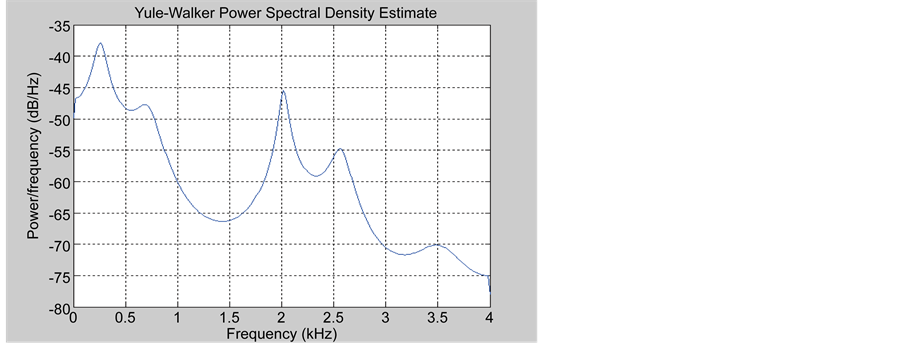
Figure 8. Estimate of the PSD (Yule Walker) the word “five”.
 (a)
(a) (b)
(b)
Figure 9. (a) Estimating the PSD (Yule Walker) in three different expressions of the word “one.”; (b) estimating the PSD (Yule Walker) in three different expressions of the word “two”.
the energy in overlapping boxes frequency of a deformed spectrum by (Mel) Frequency scale 1.
In the short term, the floor can be considered as stationary, MFCC characteristics of the vectors are calculated for each speech frame detected. Using many statements of a number and by combining all of the feature vectors, we can estimate a multidimensional probability density function (PDF) vectors to a specific figure. Repeating this process for each digit, the acoustic model is obtained for each digit. During the test phase, we extract the MFCC vectors figure test and use a probabilistic measure to determine the number of the source with the maximum likelihood.
Figure 10 shows the distribution of the first dimension of MFCC feature vectors ex-
 (a)
(a) (b)
(b)
Figure 10. (a) The distribution of the first dimension of MFCC feature vectors for the digit “one.”; (b) Overlay estimated Gaussian components (red) and all Gaussian mixture model (green) for distribution in (4a).
tracted from the training data for the digit “one.” We could use dfittool in StatisticsToolbox adapt to a PDF, but the distribution seems quite arbitrary, and standard distributions do not provide a good fit.
One solution is to adjust a mixture of Gaussian model (GMM), a sum of weighted Gaussian (Figure 10(b)). The total density of Gaussian mixture is set by the weight of the mixture, the mean vectors and covariance matrices from all densities of the components. For the recognition of isolated digits, each digit is represented by the parameters of the GMM.
To estimate the parameters of a GMM for a set of MFCC feature vectors extracted from the figure when learning, we use an expectation maximization (EM) iterative algorithm for maximum likelihood (ML) estimation. Given some MFCC training data in MFCC train data variable (equal to five here), we use the GMM distribution Statistics Toolbox function for estimating GMM parameters. This function is all that is needed to perform the EM iterative calculations.
5.2.3. Selecting a Classification Algorithm
After estimating a GMM for each digit, we have a dictionary for use in the testing phase. Given some test speech, we extracted again MFCC feature vectors of each frame of the detected word. The goal is to find the model numbers of the maximum a posteriori probability for all the long delivery tests, which reduces to maximize the value of log-likelihood.
Given a GMM model (equal to model here) model numbers and some feature vectors tests test data (equal to five here), the log-likelihood value is easily calculated using the post office in Statistics Toolbox: [P, log_like] = later (model, five); we repeat this calculation using the model of each digit. The test speech is classified as revenues at the MGM produce the maximum log-likelihood.
6. Conclusions
In this article we presented an overview of HMM: their applications and conventional algorithms used in the literature, the generation probability calculation algorithms in a sequence by an HMM, the path search algorithm optimum, and the drive algorithms.
The speech signal is a complex form drowned in the noise. Its learning is part of complex intelligent activity [10] . By learning a starting model, we will build gradually an effective model for each of the phonemes of the “Baoule” language.
Note finally that HMMs have established themselves as the reference model for solving certain types of problems in many application areas, whether in speech recognition, modeling of biological sequences or for the extraction of information from textual data. However other formalisms such as neural networks can be used to improve the modeling. Our future work will focus on the modeling of the linguistic aspect of the “Baoule” language.
Cite this paper
Konan, H., Soro, E., Asseu, O., Goore, B.T. and Gbegbe, R. (2016) Phoneme Sequence Modeling in the Context of Speech Signal Recognition in Language “Baoule”. Engineering, 8, 597-617. http://dx.doi.org/10.4236/eng.2016.89055
References
- 1. Baum, L.E., Petrie, T., Soules, G. and Weiss, N. (1970) A Maximization Technique Occurring in Statistical Analysis of Probabilistic Functions in Markov Chains. The Annals of Mathematical Statistics, 41, 164-171.
http://dx.doi.org/10.1214/aoms/1177697196 - 2. Casacuberta, F. (1990) Some Relations among Stochastic Finite State Networks Used in Automatic Speech Recognition. IEEE Ttransactions on patern Analysis and Machine Intelligence, 12, 691-695.
http://dx.doi.org/10.1109/34.56212 - 3. Lekoundji, J.-B.V. (2014) Modèles De Markov Cachés. Université Du Québec à Montréal.
- 4. Rabiner, L.R. (1989) A Tutorial on Hidden Markov Models and Selected Application in Speech Recognition. Proceedings of the IEEE, 77, 257-286.
http://dx.doi.org/10.1109/5.18626 - 5. Kundu, A., He, Y. and Bahl, P. (1988) Recognition of Handwritten Word: First and Second Order Hiden Markov Model Based Approach. IEEE Computer Society Conference on Computer Vision Pattern Recognition, CVPR’88, Ann Arbor, 5-9 June 1988, 457-462.
http://dx.doi.org/10.1109/CVPR.1988.196275 - 6. Schenkel, M., Guyon, I. and Henderson, D. (1994) On-Line Cursive Script Recognition Using Time Delay Neural Networks and Hidden Markov Models. Proceedings of 1994 IEEE International Conference on Acoustics, Speech, and Signal Processing, ICASSP’94, Adelaide, 19-22 April 1994, II-637-II-640.
http://dx.doi.org/10.1109/icassp.1994.389575 - 7. Haussler, D., Krogh, A., Mian, S. and Sjolander, K. (1992) Protein Modeling Using Hidden Markov Models: Analysis of Globins. Technical Report UCSC-CRL-92-23.
- 8. Durbin, R., Eddy, S., Krogh, A. and Mitchison, G. (1998) Biological Sequence Analysis Probabilistic Models of Proteins and Nucleic Acids. Cambridge University Press, Cambridge.
http://dx.doi.org/10.1017/CBO9780511790492 - 9. In François Le Gland (2014-2015) Télécom Bretagne Module F4B101A Traitement Statistique de l’Information.
http://www.irisa.fr/aspi/legland/telecom-bretagne/ - 10. Corge, C. (1975) Elément d’informatique. Informatique et demarche de l’esprit. Librairie Larousse, Paris.
ANNEXES
function [valeur,ante,dens] = Viterbi(X,A,p,m,sigma2,K,T)
begin
% densite d'emission
dens = ones(T,K);
dens =
exp(-0.5*(X'*ones(1,K)-ones(T,1)*m).^2./(ones(T,1)*sigma2))./sqrt(ones(T,1)*sigma2);
% fonction valeur
valeur = ones(T,K);
valeur(1,:) = p.*dens(1,:);
for t=2:T
[c,I] = max((ones(K,1)*valeur(t-1,:)).*A,[],2);
valeur(t,:) = c'.*dens(t,:);
valeur(t,:) = valeur(t,:)/max(valeur(t,:));
ante(t,:) = I;
end
end
function [alpha,beta,dens,ll] = ForwardBackward(X,A,p,m,sigma2,K,T)
% densite d'emission
dens = ones(T,K);
dens =
exp(-0.5*(X'*ones(1,K)-ones(T,1)*m).^2./(ones(T,1)*sigma2))./sqrt(ones(T,1)*sigma2);
% variable forward
alpha = ones(T,K);
alpha(1,:) = p.*dens(1,:);
c(1) = sum(alpha(1,:));
alpha(1,:) = alpha(1,:)/c(1);
for t=2:T
alpha(t,:) = alpha(t-1,:)*A;
alpha(t,:) = alpha(t,:).*dens(t,:);
c(t) = sum(alpha(t,:));
alpha(t,:) = alpha(t,:)/c(t);
end
ll = cumsum(log(c));
% variable backward
beta = ones(K,T);
for t=T-1:-1:1
beta(:,t) = beta(:,t+1).*(dens(t+1,:))';
beta(:,t) = A*beta(:,t);
beta(:,t) = beta(:,t)/(alpha(t,:)*beta(:,t));
end
function [X,Y] = gen(A,p,m,sigma2,T)
begin
sigma = sqrt(sigma2);
Y(1) = multinomiale(p);
for t=2:T
q = A(Y(t-1),:);
Y(t) = multinomiale(q);
end
w = randn(1,T);
for t=1:T
moyenne = m(Y(t));
ecart_type = sigma(Y(t));
X(t) = moyenne+ecart_type*w(t);
end
end
function Px = stpower(x,N)
begin
M = length(x);
Px = zeros(M,1);
Px(1:N) = x(1:N)'*x(1:N)/N;
for m=(N+1):M
Px(m) = Px(m-1) + (x(m)^2 - x(m-N)^2)/N;
end
end
function Zx = stzerocross(x,N)
begin
M = length(x);
Zx = zeros(M,1);
Zx(1:N+1) = sum(abs(sign(x(2:N+1)) - sign(x(1:N))))/(2*N);
for (m=(N+2):M)
Zx(m) = Zx(m-1) + (abs(sign(x(m)) - sign(x(m-1))) ...
- abs(sign(x(m-N)) - sign(x(m-N-1))))/(2*N);
end
end