Engineering
Vol.07 No.11(2015), Article ID:61614,24 pages
10.4236/eng.2015.711067
Trilinear Hexahedra with Integral-Averaged Volumes for Nearly Incompressible Nonlinear Deformation
Craig D. Foster*, Talisa Mohammad Nejad
University of Illinois at Chicago, Civil and Materials Engineering, Chicago, IL, USA

Copyright © 2015 by authors and Scientific Research Publishing Inc.
This work is licensed under the Creative Commons Attribution International License (CC BY).


Received 24 September 2015; accepted 27 November 2015; published 30 November 2015

ABSTRACT
Many materials such as biological tissues, polymers, and metals in plasticity can undergo large deformations with very little change in volume. Low-order finite elements are also preferred for certain applications, but are well known to behave poorly for such nearly incompressible materials. Of the several methods to relieve this volumetric locking, the
 method remains popular as no extra variables or nodes need to be added, making the implementation relatively straightforward and efficient. In the large deformation regime, the incompressibility is often treated by using a reduced order or averaged value of the volumetric part of the deformation gradient, and hence this technique is often termed an
 approach. However, there is little in the literature detailing the relationship between the choice of
 and the resulting
 and stiffness matrices. In this article, we develop a framework for relating the choice of
 to the resulting
 and stiffness matrices. We examine two volume-averaged choices for
 , one in the reference and one in the current configuration. Volume-averaged
 formulation has the advantage that no integration points are added. Therefore, there is a modest savings in memory and no integration point quantities needed to be interpolated between different sets of points. Numerical results show that the two formulations developed give similar results to existing methods.
Keywords:
Incompressibility, Volumetric Locking, Strain Projection, B-Bar, F-Bar, Finite Element

1. Introduction
Many materials exhibit nearly incompressible responses over some part of their deformation. Biological tissues, rubbers, metals undergoing plastic deformation, and soils under undrained conditions are examples. To model these materials in a finite element (FE) context, care has to be taken to use elements designed for nearly incompressible behavior. The fact that low-order finite elements perform poorly for nearly incompressible media is well known, and treatment for this issue has received significant attention. There are several ways to view the problem, but one is that standard elements have too many incompressibility constraints which overwhelm the shear response. While higher-order elements can relieve this, even they do not behave optimally. And for certain classes of problems, such as some dynamic problems or problems involving jumps in the displacement field, low-order elements are generally preferred.
Many solutions have been proposed to relieve this volumetric locking effect in low-order elements, particularly quadrilaterals and hexahedra. Reduced integration [1] can reduce the number of volumetric constraints, but results in spurious non-zero energy modes are often called hourglass modes. However, modification can control these modes ( [2] - [5] , among others). Mixed methods treat the mean stress as a separate variable. While effective, the extra set of equations complicates the process and results in higher computation time (see [6] - [9] among others). It should be noted that many times the extra variable may be condensed at the element level, minimizing this extra cost. Assumed enhanced strain formulations add extra terms to the strain and can relieve locking, for example in [10] [11] . Variational multiscale methods [12] - [14] , and other stabilization techniques ( [15] among others) have also been employed to relieve locking, but also add extra complexity to the system.
Because they can be implemented relatively simply in a displacement-only framework, the so-called
 methods have been highly popular. Discussed in [16] for linear elements, these elements replace the volumetric part of the strain-displacement matrix with a reduced-order integration or averaged value. The reduced interpolation order of the volumetric term reduces the number of constraints, relieving the locking. No extra degrees of freedom are added to the system, though in some cases additional integration points are added. While these elements do not formally satisfy the Ladyzenskaya-Babuska-Brezzi stability conditions [17] [18] , they perform well in practice and their relative ease of implementation has made the approach popular.
For the finite deformation case, these methods have been extended using a so-called
 approach. This approach takes a reduced order or average evaluation of the deformation gradient
 . Several variations on this idea have been proposed, including reduced integration scheme for the logarithm of the volumetric deformation [19] , reduced integration scheme for the volumetric deformation [20] [21] , and an average over the element reference volume of the Jacobian [22] . In another approach, modified Jacobian
 is defined by relating it to a volume change parameter [23] . Most authors choose to use the
 modification for the gradient of the weighting function (virtual velocity gradient), though some do not [20] [21] . While it has not been emphasized in the literature, each choice of
 yields a corresponding
 matrix, which in general has a different averaging scheme than the
 . Many authors also do not comment on the stiffness matrix.
In this paper, we develop an 8-node hexahedral element that averages the Jacobian over the element. While the integration procedure adds some modest complexity to the computation time to the code, it avoids tracking variables at an extra integration point. Extra integration points can add memory costs. They can also add significant complexity in multiphysics problems or history-dependent materials, though we do not investigate those here. We examine integral averages in both the reference and current configurations, and detail the relationship between the choice of
 and
and , as well as explicitly deriving the stiffness matrix.
While beyond the scope of this paper, it bears mentioning that the
 method does not work for linear triangles and tetrahedra, as the volumetric deformation is already constant in the element. However, the concepts have been extended to these elements using a method termed “
 -patch”, where the volumetric deformation is taken as not constant over a single element, but a small patch of contiguous elements [24] . Recently, a
 approach has been applied to NURBS-based finite elements as well [23] [25] .
The remainder of the paper is organized as follows: Section 2 discusses integral averages for , including two of several possible choices. Section 3 derives the
 formulation consistent with the choice of
 . The stiffness matrix is presented in Section 4, though the full derivation is relegated to the Appendix. This section is followed by numerical examples and, finally, some conclusions.
Notation
A few notes on notation: We employ the summation convention in this paper, that a repeated index within a single term of an expression has an implied sum over the range of the index. For example , where
 is the trace operator, and
 is equivalent to
 .
.
Outer products are represented with the ‘ ’ symbol, e.g. for two matrix
 and
and ,
, . For a matrix
 and vector
 ,
,
 , and for two vectors
 and
and ,
, .
.
First- and second-order tensors are denoted in bold, e.g.
 or
or . Third-order tensors of matrices are written in calligraphic script, for example,
 , and fourth-order tensors in blackboard bold, such as
 .
.
We use curly braces for second-order tensors converted to vectors in Voigt notation. Kinematic quantities have doubled off-diagonal terms unless stated otherwise, while other quantities do not. For example
 . (1)
. (1)
Similarly, fourth-order tensors converted to Voigt-form matrices are denoted with brackets, e.g. .
.
2.
 Formulations
The basis of the
 formulation for geometrically nonlinear material models is to replace the dependence of the stress on the deformation gradient
 with a dependence on a modified deformation gradient
 , e.g.
 . (2)
. (2)
Here,
 is the Kirchhoff stress, though the use of any stress measure may suffice. The ellipsis is a reminder that the stress may also be a function of the rate of deformation, internal state variables, or other quantities. To relieve volumetric locking associated with nearly incompressible materials, typically the volumetric part of
 is replaced by an average or reduced order approximation. To accomplish this task,
 is typically split into a volumetric component
 and an isochoric component
 such that
 (3)
(3)
where
 is the second order identity tensor and
 is the Jacobian of the deformation. The Jacobian, then, is replaced with some modified
 , resulting in a modified deformation gradient
 . (4)
. (4)
Many forms for
 have been proposed. Effective choices should reduce the order of the volumetric strain interpolation to reduce the number of volumetric constraints. One of the simplest for trilinear hexahedra (and their two-dimensional counterparts, the bilinear quadrilaterals) is to evaluate the modified Jacobian at the center of the element,
 , for example as a case of [19] . The drawback of this approach is that the deformation must be evaluated at an extra Gauss point. This extra data modestly increases memory requirements and increases the complexity of the code. The complexity increases for more sophisticated constitutive models such as plasticity models, where internal state variables and other quantities must be tracked, and multiphysics formulations, where mechanical quantities must be shared with quantities from the other physics.
An alternative approach is to use an averaging scheme or stabilization procedure. We adopt the former in the paper. Specifically, we examine two possibilities
 (5)
(5)
and
 . (6)
. (6)
The first is a volume average of the Jacobian over the reference volume of the element , the second a volume average over the current element volume
 . Since the reference configuration is at times an arbitrary theoretical state, there is some logic to adopting the second. However, the formulation for the former, we will see, is simpler, and for nearly incompressible materials, there is not a great difference between the volume in the current and reference configurations.
Note: As discussed in [19] , for very nearly or completely incompressible materials, hourglass modes may appear due to ill-conditioning of the stiffness matrix. These modes can be alleviated by replacing
 with an
 , composed of
 and
and . The authors in [19] use
 , for some relatively small
 (originally suggested in [26] ). Similarly, Doll and coworkers [27] proposed a
 . For models which use a volumetric penalty parameter, however, these modes may also be eliminated by setting the volumetric penalty stiffness not too much higher than the shear stiffness. We do not perform a formal analysis of appropriate penalty parameter values in this paper, but roughly three to four orders of magnitude higher than shear stiffness parameters appear to be an appropriate value in practice.
3. Consistent
 Formulations
The appropriate function for the
 follows from the chosen form for
 . One can derive the standard
 matrix from the velocity gradient
 using a pseudo-time derivative, as shown in [28] . In a finite element context
 (7)
(7)
where
 in this paper refers to the vector of element nodal displacements (we have dropped the common superscript
 to simplify the notation). We adopt a similar approach to derive
 , i.e.
 . (8)
. (8)
First, we must derive an expression for the modified velocity gradient

 (9)
(9)
 . (10)
The expression for
 can be determined as
 (11)
(11)
 (12)
(12)
 (13)
(13)
 (14)
(14)
 . (15)
Here we define . This quantity will depend, of course, on the choice of
 . We derive this quantity in a moment for the choices we have considered, but first note that for any choice of

 (16)
(16)
 (17)
(17)
 (18)
(18)
 . (19)
Note that this has the familiar form of the small strain
 formulation where the trace of the small strain tensor is replaced with the modified component.
For the choice of ,
,
 (20)
(20)
 (21)
(21)
 . (22)
Hence
 (23)
(23)
 . (24)
Curiously, averaging J over the reference configuration results in
 being averaged over the current configuration.
Averaging J over the current configuration results in a somewhat more complicated formulation. In this case
 (25)
(25)
 (26)
(26)
 (27)
(27)
 (28)
(28)
 (29)
(29)
 . (30)
Hence
 . (31)
In a finite element context, we can factor out the element nodal velocity vector implicit in the equations from the finite element shape functions. Recall that
 (32)
(32)
 (33)
(33)
where
 is the ith degree of freedom for element nodal displacement subvector
 . The
. The
 operator in the paper is used with respect to the current coordinates. Therefore
 (34)
(34)
 (35)
(35)
 . (36)
Here,
 is the third-order tensor that relates the velocity gradient to the nodal velocity subvector
 .
.
 . (37)
In other words, it is the tensor equivalent of the standard updated Lagrangian
 matrix (see, for example, [28] ). For a given choice of
 , we need only calculate the appropriate
 . For the Jacobian averaged over the reference configuration
 (38)
(38)
 (39)
(39)
 (40)
(40)
 (41)
(41)
where
 (42)
(42)
Similarly, for the Jacobian averaged in the current configuration
 (43)
(43)
 (44)
(44)
 . (45)
Therefore
 . (46)
With the correct expression for , we can write
 . (47)
In implementation, this expression is generally rearranged into a vector form such that
 . (48)
In this case, the nodal submatrix
 takes the form
 (49)
(49)
The full
 may be written as usual as
 (50)
(50)
where
 is the number of element nodes (8 in this case, but we keep the notation for generality).
We assume that the gradient of the weighting function, or virtual velocity vector, takes the same modifications as that used in the physical velocity gradient. Hence the element internal force vector may be written
 . (51)
This derivation may also be carried out in a total Lagrangian setting, however, the volumetric part does not separate out as cleanly and the formula is more complicated.
Note: It is not strictly necessary to use the same averaging for the virtual velocity gradient as for the actual, or, in fact, any averaging. The authors in [20] use the standard
 matrix for the virtual velocity gradient, i.e.
 . (52)
The resulting formulation is somewhat simpler, but is also nonsymmetric. As the authors point out in that article, some materials have a nonsymmetric tangent stiffness already, and for these materials little is lost. However, for materials with a symmetric tangent stiffness, the proposed formulation creates a symmetric stiffness matrix, which has advantages in storage and solution time.
4. Stiffness Matrix
The stiffness matrix may be derived by taking a directional derivative, or another pseudo-time derivative. The derivation is relegated to the appendix, where the latter approach is taken. If
 is the number of degrees of freedom per node, the
 nodal submatrix
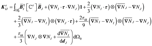
 of stiffness matrix relating the residual vector for node I to the displacements at node J has the form
 (53)
(53)
where
 is the tangent modulus between the convected rate of the Kirchhoff stress and the rate of deformation tensor, i.e.
 [28] .
The formula is general, and can be applied for any choice of . One simply has to calculate the derivative
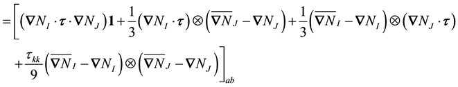
 . For the Jacobian averaged in the reference configuration
 . (54)
For the Jacobian averaged in the current configuration
 . (55)
Clearly the second formula is more complex than the first. These formulas are derived in the appendix.
5. Numerical Examples
In this section, the performance of the proposed
 method is investigated by means of numerical examples. Four numerical examples with nearly incompressible nonlinear elastic material properties are presented.
5.1. Three-Dimensional Block
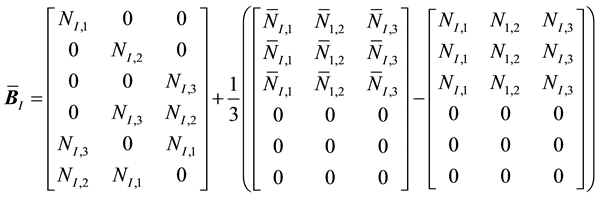
In the first three numerical examples, a nearly incompressible nonlinear elastic block fixed on bottom and subjected to three different loading conditions are presented. The block is 2 meters high with a square cross section of 1 meter, shown in Figure 1. The quantity we compare is the displacement at node A located at (1, 2, 1) meters.
For this set of examples, the material model used is a Neo-Hookean model that follows the decomposition of strain energy function into isochoric and volumetric components:
 (56)
(56)
in which U is the penalty function enforcing incompressibility defined as
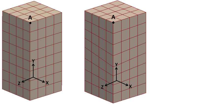
Figure 1. Geometry of a block with 2 m height and a square cross section of 1 square meter. The block is meshed with 128 regular hexahedra (i.e. cubes) on the left and 128 irregular hexahedra on the right. We focus on comparing the displacement at node A using standard and
 trilinear hexahedral elements under different loading conditions.
 (57)
(57)
where K is a generalization of the linear bulk modulus. The isochoric part may be defined as
 . (58)
In which
 is analogous to the shear modulus and
 is the first invariant of the modified right Cauchy-Green deformation tensor defined as
 . (59)
The material parameters of
 and
and
 are used.
This set of examples investigates the performance of three-dimensional mean dilatation 8-node
 hexahedral elements employed in our large deformation FE computer code under a side pressure, compressive pressure and specified tensile displacement. The obtained displacement results are then compared to standard 8-node hexahedral elements and 8-node hexahedral
 elements used in ANSYS (Solid 185) for verification. Solid 185 is an 8-node hexahedral element that has large deformation capabilities and can be used in 3-dimensional simulation of fully incompressible hyperelastic models. We use the default
 option that employs “selective reduced integration”.
5.1.1. Block Subjected to Side Pressure
This example is used to assess performance of near incompressible limit material subjected to a side pressure. Follower forces are used. In this block, displacement is fully constrained in bottom and a side pressure of 2 kPa is uniformly applied to the front left edge. Three meshes respectively consisting of 2, 16 and 128 elements are considered to investigate the convergence. For each mesh, the solution for the two element shapes is obtained to ensure that elements with nonconstant initial element Jacobians perform well (for clarity, the element Jacobian is the volume ratio between the physical volume and the volume in the bi-unit cube in the parent domain, and is different from the Jacobian of the deformation which we have been discussing throughout this paper). For each mesh, regular and irregular hexahedra, and each refinement, four cases are run: standard displacement elements with no special treatment of the volumetric deformation,
 elements with the Jacobian averaged in the reference configuration,
 elements with the Jacobian averaged in the current configuration, and ANSYS Solid 185 elements. The displacement results at node A located at (1, 2, 1) meters are obtained for each approach and compared in Table 1. The convergence as a function of the number of elements per mesh is investigated.
From the obtained results we can see that average volume
 elements improve the displacement results over standard methods in the analysis of large deformation nearly incompressible materials. The displacement results obtained from both of the proposed
 approaches closely agree with ANSYS large deformation
 method. Convergence of solution with mesh refinement is also observed. The deformed shapes are shown in Figure 2. Since refinement, perturbations in element shape, and type of averaging are satisfied, for remaining examples we run only the irregular, 128-element mesh with the reference-averaged Jacobian.
Table 2 illustrates the evolution of the norm of the residual over the iterations for the last loading step for
 averaged in the reference configuration. The results indicate that the proposed tangent matrix leads to quadratic convergence rate.

Figure 2. Deformed shape of an incompressible block subjected to side pressure and fixed bottom displacement obtained from FE simulation using (a) standard 8-node hexahedral elements (b) mean- dilatational 8-node
 cubes elements (c) mean-dilatational 8-node
 irregular hexahedral elements. In cases (b) and (c), the deformation is shown for J averaged in the reference configuration, but all the
 methods exhibited very similar deformation. The wireframe in black is the undeformed mesh and the solid surface with red wireframe shows the deformed shape of the block.

Table 1. Displacement results, in m, obtained at node A, using standard and
 FE method for different numbers of elements per mesh.
Table 2. Evolution of the residual norm during the last time step in Newton-Raphson iterations with the proposed
 approach.
5.1.2. Block Subjected to Compressive Pressure
This example is presented to assess performance of the proposed
 approach in simulation of a block with near incompressible limit material properties under a compressive pressure. The displacement of the block is fully constrained on the bottom, and a pressure of 12 kPa is uniformly applied to the top surface. The solution is obtained for the 128-element mesh with irregular hexahedra using 3 different element types: standard 8-node hexahedral elements, the proposed mean-dilatation
 8-node hexahedral elements with J averaged in the reference configuration, and 8-node hexahedral
 elements employed in ANSYS. Displacement results obtained from 3 approaches at node A are displayed in Table 3. The displacement results obtained with the proposed
 approach almost match the ones obtained using ANSYS trilinear hexahedra. The deformed shape of the block under compression is also depicted in Figure 3.
As illustrated in this figure and the table, displacement results are larger with
 elements than with standard elements. The two
 methods are quite comparable. As expected, the deformation
 schemes confirm that they relieve the volumetric locking behavior in the analysis of nearly incompressible materials.
5.1.3. Block Subjected to Tensile Displacement
In this example, performance of the proposed
 approach in the simulation of a nearly incompressible block under tension is assessed. The top surface of the block is given a uniform tensile displacement of 0.4 meters and the deformation is fully constrained in bottom. The displacement solution is obtained for a 128-element mesh of irregular hexahedra using 3 different element types: standard 8-node hexahedral elements, proposed mean-dilatation 8-node hexahedral
 elements with the Jacobian averaged in the reference configuration, and 8-node
 hexahedral elements employed in ANSYS. For standard and the proposed
 approach, the deformed shape is displayed in Figure 4. The displacements of the block are magnified by a factor of two in order to better visualize the volumetric locking in standard finite elements. In addition to locking, the standard mesh with irregular elements produces a notable asymmetry in the response. Figure 5 and Figure 6 respectively illustrate the distribution of vertical and von Mises Kirchhoff stresses, respectively, on the block. Figure 7 depicts the plot of reaction force versus displacement using standard and
 trilinear elements. As shown in that graph, using standard finite elements for nearly incompressible materials results in greater resistance to external displacement due to the tendency to lock.
5.2. Cook’s Membrane
Cook’s membrane is a classical plane strain problem used to test performance of elements in nearly incompressible problems under moderate distortion. Here we apply the problem in three dimensions, with one layer of elements in depth and all nodes constrained out of plane. We follow the nonlinear example in [29] , using the Neo-Hoo-kean potential in the previous examples, which is identical to the one is used in that paper.
The geometry is shown in Figure 8, and an upward load of 1 N is distributed evenly across the right hand side. Again following [29] , we use
 N/mm2, and
 N/mm2.
We compare meshes of 16, 64, and 256 elements. The deformed meshes for the standard and
 cases for 256 elements are shown in Figure 9. As is well known, the standard case shows far less deformation, and little shear stress related to bending. The
 cases show a more complete deformation pattern.
For quantitative comparison, the vertical displacements at the upper right node are recorded. For verification, ANSYS is again run with the Solid 185 element. The results are shown in Table 4. The results between the ANSYS solution and our
 formulation are very close. These results also compare quite well with [29] .

Figure 3. Deformed shape of an incompressible block subjected to uniform pressure on top and fixed displacement on bottom obtained from FE simulation using standard 8-node hexahedral elements (on the left) and mean-dilatational 8-node
 hexahedral elements (on the right). The solid surface with red wireframe is the undeformed shape and the wireframe in black shows the deformed shape.
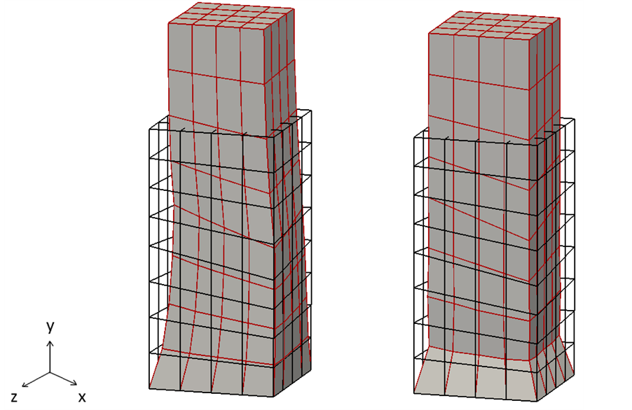
Figure 4. Deformed shape of an incompressible block subjected to uniform tensile displacement on top and fully restricted displacement on bottom, obtained from FE simulation using standard 8-node hexahedral elements (on the left) and mean-dilatational 8-node
 hexahedral elements (on the right). The wireframe in black is the undeformed mesh and the solid surface with red wireframe shows the deformed shape of the block, with displacements magnified by a factor of two.
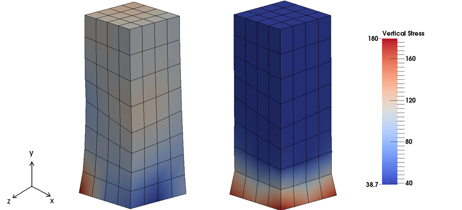
Figure 5. Distribution of Kirchhoff vertical stress τyy obtained from FE simulation using standard 8-node hexahedral elements (on the left) and mean-dilatational 8-node
 hexahedral elements (on the right). The tensile stress is notable higher in the standard example.
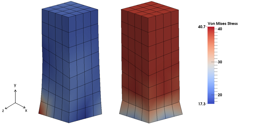
Figure 6. Distribution of Kirchhoff von Mises stress obtained from FE simulation using standard 8-node hexahedral elements (on the left) and mean-dilatational 8-node
 elements (on the right).
Table 3. Displacement results for the block in compression obtained at node A using standard and
 elements under compressive pressure.
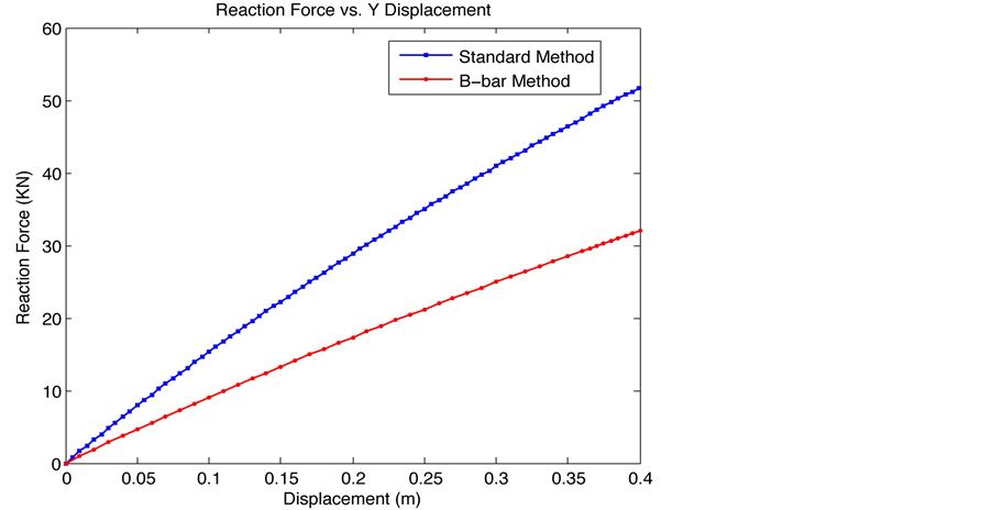
Figure 7. Plot of the reaction force versus displacement using standard and
 trilinear hexahedral elements for the block under prescribed tensile dis- placement.
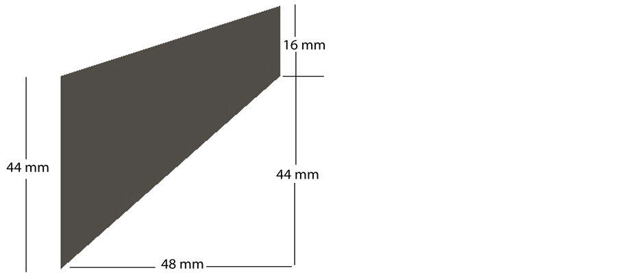
Figure 8. Geometry for Cook’s membrane problem. The model is one mm out of plane, with no deformation allowed in the out-of-plane direction.
Table 4. Vertical displacement results, in mm, at top right node, using standard and
 FE method for different numbers of elements per mesh.
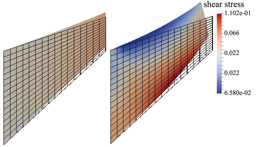
Figure 9. Deformed shapes for both standard integration (left) and
 cases, with in-plane shear stress shown. The undeformed mesh is shown in black wireframe.
5.3. Incompressible Mouse Cornea Subjected to Pressure
In the final example, the incompressible behavior of a three-dimensional mouse cornea subjected to pressure loading is studied by means of standard and
 methods. Biological tissues are prime examples of nearly incompressible media, and the current approach has been applied with good results in [30] [31] . An intraocular pressure of 1.73 kPa is applied to the posterior side of the cornea. The cornea displacement but not rotation is restricted along the center of the cornea edge. While some models of the human cornea use more restrictive boundary conditions on the edges, the mouse cornea is thinner at the edge than at the center, and hence the approximation used here is appropriate. Four different meshes each having 2, 4, 6, and 8 layers of elements through the cornea thickness consisting of respectively 1360, 2720, 4080, and 5440 hexahedral elements are considered to assess convergence.
The mouse cornea is a nearly incompressible soft biological tissue consisting of five layers of which the stroma is the thickest and stiffest. For simplicity, only the stiffness of the stroma is considered in the constitutive model development. The stroma is composed of oriented and dispersed collagen fibrils embedded in nearly incompressible matrix. The material model used is an anisotropic hyperelastic model adapted from Pandolfi and Holzapfel [32] for the human cornea. The model follows the decomposition of the strain energy function into an isochoric component and volumetric components of oriented fibrils distributed in Neo-Hookean matrix:
 (60)
(60)
in which U is the penalty function enforcing incompressibility constraints of the cornea defined as
 (61)
(61)
where
 is a positive penalty parameter. The isochoric component may be written
 (62)
(62)
 (63)
(63)
 (64)
(64)
 (65)
(65)
 (66)
(66)
for a given unit orientation vector . Here
 is the shear modulus analogue for the matrix and
 and
and
 are materials parameters that define the stiffening effect of the fibrils. The values of the material parameters used in the simulation are given in Table 5.
The unit vector
 is the mean orientation of collagen fibrils in the reference configuration. For the human cornea, fibrils are characterized by two mean orientations [32] . However, based on x-ray images [33] , one mean orientation of collagen fibrils is assumed for the mouse cornea and accordingly the quantities involving
 are removed from the constitutive equations presented in [32] . The mean orientation is assumed to be horizontal (nasal-temporal) near the center, and circumferential near the edge. There is a transition region in between, where the orientation is linearly interpolated. The dispersion parameter
 describes the ratio of anisotropic fibrils to isotropically distributed ones in the cornea. For the mouse cornea, in the region around the cornea center, we assume that approximately 80% of collagen fibrils are oriented in horizontal direction and 90% have cir-
cumferential orientation around the cornea edge. Again, in the transition region, a linear interpolation of the two directions is assumed.
Spheres with different radii of curvature for outer and inner surfaces of the cornea result in varying thickness throughout. For the mouse cornea model, a thickness of 0.3 mm at the apex and 0.1 mm at the edge was assumed. An initial cornea height of 0.84 mm and the distance from cornea center to the inner and outer edges of respectively 1.33 mm and 1.39 mm were used.
The finite element simulation is performed using the standard 8-node hexahedral elements and the proposed
 approach, with J averaged in the reference configuration. The convergence is studied by increasing the number of layers of elements through the thickness of the mesh. The quantity of interest is the displacement in the vertical direction at the corneal apex.
The results of vertical displacement at the apex versus the number of element layers through corneal thickness are shown in Figure 10. The results obtained with standard 8-node hexahedral elements and with 8-node
 elements are compared. Using the
 method, all the displacement values reach a converged solution with
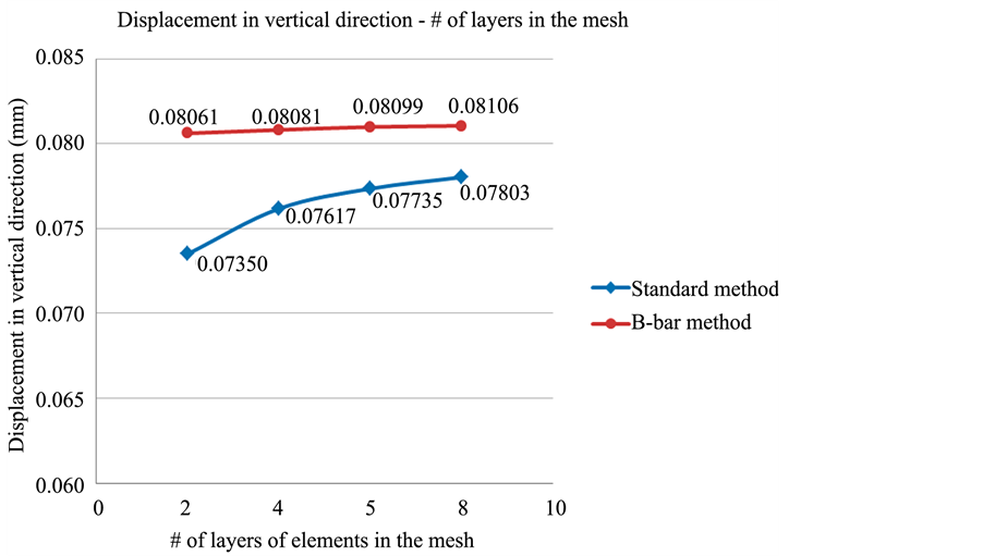
Figure 10. Vertical Displacement at the cornea apex versus number of layers of elements through the corneal thickness with standard and
 elements obtained from nonlinear and anisotropic FE simulations of mouse cornea subjected to intraocular pressure.
fewer layers, and the standard elements appear to exhibit some locking. Figure 11 also illustrates the deformed shape of the cornea using the standard and
 FE simulation. This example demonstrates that the proposed method functions well even with anisotropic materials.
6. Conclusions
In summary, we have developed a
 method for finite deformation nearly incompressible materials, based on an integral average of the volumetric part of the deformation gradient. There is an advantage in such formulations over reduced-order quadrature formulation in that the deformation can be tracked at fewer integration points, saving memory and perhaps, modestly, computation time. Though not considered here, the advantages are greater in history-dependent materials and multiphysics applications. While integral-averaged
 methods have been proposed before, there appears to be little in the literature linking a given choice of
 to the appropriate
 matrix in these cases, especially for integral formulations. The consistently derived stiffness also ap- pears to be lacking in most of the literature for integral-averaged
 formulations in standard finite elements, though it has been derived reduced-order quadrature formulations.
We have examined two possible choices for the integral averaging of the Jacobian, over the reference configuration and over the current configuration. While there may be some justifications for the current configuration as more natural, the formulation is more complex. Since the volume change in nearly incompressible materials
Table 5. Material constants assumed for anisotropic and nonlinear FE simulation of mouse cornea.
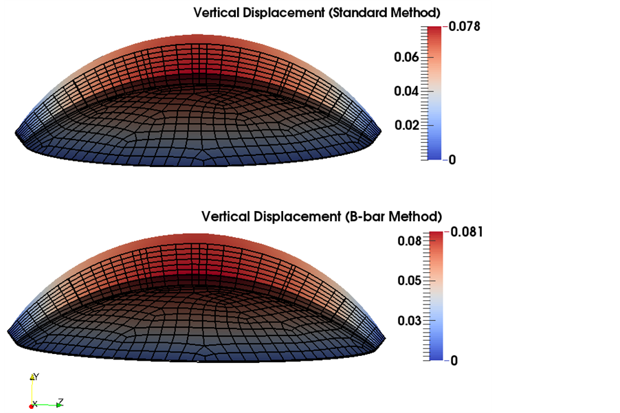
Figure 11. Vertical displacement mapping of a mouse cornea subjected to pressure obtained from standard and
 FE simulation (the top and bottom figures respectively) are shown in cross section. The wireframe on the bottom is the undeformed mesh and vertical displacement colored by magnitude is shown on top. The cornea displacement but not rotation is restricted along the center of the cornea edge.
is small, one does not expect there to be a great difference in the results. This observation is confirmed by numerical examples.
Since the formulation is general, it can be applied to other choices of , including reduced integration or logarithmic variations. The formulation is not limited to isotropic materials and can be extended to inelastic materials with some work. Overall, numerical results are similar to existing
 methods.
Acknowledgements
The authors gratefully acknowledge the support of the U.S. National Institutes of Health grant 1R21EY020946- 01.
Cite this paper
Craig D.Foster,Talisa MohammadNejad, (2015) Trilinear Hexahedra with Integral-Averaged Volumes for Nearly Incompressible Nonlinear Deformation. Engineering,07,765-788. doi: 10.4236/eng.2015.711067
References
- 1. Hughes, T.J.R. (1987) The Finite Element Method. Prentice-Hall, Upper Saddle River.
- 2. Flanagan, D.P. and Belytschko, T. (1981) A Uniform Strain Hexahedron and Quadrilateral with Orthogonal Hourglass Control. International Journal for Numerical Methods in Engineering, 17, 679-706.
http://dx.doi.org/10.1002/nme.1620170504 - 3. Belytschko, T., Ong, J.S.J., Liu, W.K. and Kennedy, J.M. (1984) Hourglass Control in Linear and Nonlinear Problems. Computer Methods in Applied Mechanics and Engineering, 43, 251-276.
http://dx.doi.org/10.1016/0045-7825(84)90067-7 - 4. Reese, S., Kussner, M. and Reddy, B.D. (1999) A New Stabilization Technique for Finite Elements in Non-Linear Elasticity. International Journal for Numerical Methods in Engineering, 44, 1617-1652.
http://dx.doi.org/10.1002/(SICI)1097-0207(19990420)44:11<1617::AID-NME557>3.0.CO;2-X - 5. Reese, S., Wriggers, P. and Reddy, B.D. (2000) A New Locking-Free Brick Element Technique for Large Deformation Problems in Elasticity. Computers & Structures, 75, 291-304.
http://dx.doi.org/10.1016/S0045-7949(99)00137-6 - 6. Sussman, T. and Bathe, K.J. (1987) A Finite Element Formulation for Nonlinear Incompressible Elastic and Inelastic Analysis. Computers & Structures, 26, 357-409.
http://dx.doi.org/10.1016/0045-7949(87)90265-3 - 7. Chapelle, D. and Bathe, K.J. (1993) The Inf-Sup Test. Computers & Structures, 47, 537-545.
http://dx.doi.org/10.1016/0045-7949(93)90340-J - 8. Kasper, E.P. and Taylor, R.L. (2000) A Mixed-Enhanced Strain Method Part I: Geometrically Linear Problems. Computers & Structures, 75, 237-250.
http://dx.doi.org/10.1016/S0045-7949(99)00134-0 - 9. Kasper, E.P. and Taylor, R.L. (2000) A Mixed-Enhanced Strain Method Part II: Geometrically Nonlinear Problems. Computers & Structures, 75, 251-260.
http://dx.doi.org/10.1016/S0045-7949(99)00135-2 - 10. Simo, J.C., Taylor, R.L. and Pister, K.S. (1985) Variational and Projection Methods for the Volume Constraint in Finite Deformation Elasto-Plasticity. Computer Methods in Applied Mechanics and Engineering, 51, 177-208.
http://dx.doi.org/10.1016/0045-7825(85)90033-7 - 11. Simo, J.C. and Rifai, M.S. (1990) A Class of Mixed Assumed Strain Methods and the Method of Incompatible Modes. International Journal for Numerical Methods in Engineering, 29, 1595-1638.
http://dx.doi.org/10.1002/nme.1620290802 - 12. Masud, A. and Xia, K.M. (2005) A Stabilized Mixed Finite Element Method for Nearly Incompressible Elasticity. Journal of Applied Mechanics-Transactions of the ASME, 72, 711-720.
http://dx.doi.org/10.1115/1.1985433 - 13. Masud, A. and Xia, K.M. (2006) A Variational Multiscale Method for Inelasticity: Application to Superelasticity in Shape Memory Alloys. Computer Methods in Applied Mechanics and Engineering, 195, 4512-4531.
http://dx.doi.org/10.1016/j.cma.2005.09.014 - 14. Xia, K.M. and Masud, A. (2009) A Stabilized Finite Element Formulation for Finite Deformation Elastoplasticity in Geomechanics. Computers and Geotechnics, 36, 396-405.
http://dx.doi.org/10.1016/j.compgeo.2008.05.001 - 15. Ramesh, B. and Maniatty, A.M. (2005) Stabilized Finite Element Formulation for Elastic-Plastic Finite Deformations. Computer Methods in Applied Mechanics and Engineering, 194, 775-800.
http://dx.doi.org/10.1016/j.cma.2004.06.025 - 16. Hughes, T.J.R. (1980) Generalization of Selective Integration Procedures to Anisotropic and Nonlinear Media. International Journal for Numerical Methods in Engineering, 15, 1413-1418.
http://dx.doi.org/10.1002/nme.1620150914 - 17. Brezzi, F. and Fortin, M. (1991) Mixed and Hybrid Finite Element Methods. Springer, Berlin, Heidelerg and New York.
http://dx.doi.org/10.1007/978-1-4612-3172-1 - 18. Szabo, B. and Babuska, I. (1991) Finite Element Analysis. Wiley, New York.
- 19. Moran, B., Ortiz, M. and Shih, C.F. (1990) Formulation of Implicit Finite-Element Methods for Multiplicative Finite Deformation Plasticity. International Journal for Numerical Methods in Engineering, 29, 483-514.
http://dx.doi.org/10.1002/nme.1620290304 - 20. de Souza Neto, E.A., Peric, D., Dutko, M. and Owen, D.R.J. (1996) Design of Simple Low Order Finite Elements for Large Strain Analysis of Nearly Incompressible Solids. International Journal of Solids and Structures, 33, 3277-3296.
http://dx.doi.org/10.1016/0020-7683(95)00259-6 - 21. de Souza Neto, E.A., Peric, D. and Owen, D.R.J. (2008) Computational Methods for Plasticity. Wiley, New York.
http://dx.doi.org/10.1002/9780470694626 - 22. Nagtegaal, J.C., Parks, D.M. and Rice, J.R. (1974) On Numerically Accurate Finite Element Solutions in the Fully Plastic Range. Computer Methods in Applied Mechanics and Engineering, 4, 153-177.
http://dx.doi.org/10.1016/0045-7825(74)90032-2 - 23. Mathisen, K.M., Okstad, K.M., Kvamsdal, T. and Raknes, S.B. (2011) Isogeometric Analysis of Finite Deformation Nearly Incompressible Solids. Journal of Structural Mechanics, 44, 260-278.
- 24. de Souza Neto, E.A., Pires, F.M.A. and Owen, D.R.J. (2005) F-Bar-Based Linear Triangles and Tetrahedral for Finite Strain Analysis of Nearly Incompressible Solids. Part I: Formulation and Benchmarking. International Journal for Numerical Methods in Engineering, 62, 353-383.
http://dx.doi.org/10.1002/nme.1187 - 25. Elguedj, T., Bazilevs, Y., Calo, V.M. and Hughes, T.J.R. (2008) F-Bar Projection Method for Finite Deformation Elasticity and Plasticity Using NURBS Based Isogeometric Analysis. International Journal of Material Forming, 1, 1091- 1094.
http://dx.doi.org/10.1007/s12289-008-0209-7 - 26. Belytschko, T., Tsay, C.S. and Liu, W.K. (1981) A Stabilization Matrix for the Bilinear Mindlin Plate Element. Computer Methods in Applied Mechanics and Engineering, 29, 313-327.
http://dx.doi.org/10.1016/0045-7825(81)90048-7 - 27. Doll, S., Schweizerhof, K., Hauptmann, R. and Freischläger, C. (2000) On Volumetric Locking of Low-Order Solid and Solid-Shell Elements for Finite Elastoviscoplastic Deformations and Selective Reduced Integration. Engineering Computations, 17, 874-902.
http://dx.doi.org/10.1108/02644400010355871 - 28. Belytschko, T., Liu, W.K. and Moran, B. (2000) Nonlinear Finite Elements for Continua and Structures. John Wiley & Sons, New York.
- 29. Brink, U. and Stein, E. (1996) On Some Mixed Finite Element Methods for Incompressible and Nearly Incompressible Finite Elasticity. Computational Mechanics, 19, 105-119.
http://dx.doi.org/10.1007/BF02824849 - 30. Rhee, J., Nejad, T.M., Comets, O., Flannery, S., Gulsoy, E.B., Iannaccone, P. and Foster, C. (2015) Promoting Convergence: The Phi Spiral in Abduction of Mouse Corneal Behaviors. Complexity, 20, 22-38.
http://dx.doi.org/10.1002/cplx.21562 - 31. Nejad, T.M., Iannaccone, S., Rutherford, W., Iannaccone, P.M. and Foster, C.D. (2015) Mechanics and Spiral Formation in the Rat Cornea. Biomechanics and Modeling in Mechanobiology, 14, 107-122.
http://dx.doi.org/10.1007/s10237-014-0592-6 - 32. Pandolfi, A. and Holzapfel, G.A. (2008) Three-Dimensional Modeling and Computational Analysis of the Human Cornea Considering Distributed Collagen Fibril Orientations. Journal of Biomechanical Engineering-Transactions of the ASME, 130, Article ID: 061006.
http://dx.doi.org/10.1115/1.2982251 - 33. Sheppard, J., Hayes, S., Boote, C., Votruba, M. and Meek, K.M. (2010) Changes in Corneal Collagen Architecture during Mouse Postnatal Development. Investigative Ophthalmology & Visual Science, 51, 2936-2942.
http://dx.doi.org/10.1167/iovs.09-4612
Appendix 1: Stiffness Derivation
As mentioned previously, the stiffness matrix may be derived using a directional derivative or a pseudo-time derivative. Here, we take the latter approach. We examine the nodal subvector of the element internal force vector
 (67)
(67)
where, as mentioned previously,
 and
and . For preliminaries, note that
 (68)
(68)
 (69)
(69)
 (70)
(70)
 (71)
(71)
 . (72)
For convenience, for the remainder of the derivation, we will move the nodal subscript of the
 and
and
 tensors to superscripts, e.g.
 . Next,
 (73)
(73)
 (74)
(74)
 . (75)
The time derivative of the nodal subvector of the element internal force vector, then, can be written
 . (76)
Examining the quantity inside the integral
 . (77)
We examine the second term first. Recall that
 is a function of
 rather than
 . Hence,
 (78)
(78)
rather than . Continuing
 (79)
(79)
 (80)
(80)
 (81)
(81)
 (82)
(82)
 . (83)
Taking the second and third quantities one at a time
 (84)
(84)
 (85)
(85)
 (86)
(86)
 . (87)
The third quantity becomes
 (88)
(88)
 (89)
(89)
 (90)
(90)
 . (91)
Next we evaluate
 (92)
(92)
 (93)
(93)
 (94)
(94)
 . (95)
Adding up all these quantities, we find that
 (96)
(96)
and hence the nodal submatrices of the element stiffness matrix may be written
 . (97)
The first term is the common “material stiffness” with the modified
 matrix, and the second term the standard geometric stiffness. The remaining terms arise from the modifications to the derivatives introduced by modifying the
 matrix. The final term, of course, depends on the form of
 . For the Jacobian averaged over the reference configuration
 (98)
(98)
 (99)
(99)
 (100)
(100)
 (101)
(101)
 (102)
(102)
 . (103)
Therefore,
 . (104)
The process for the Jacobian averaged in the current configuration is the same, though the calculations are more tedious.
 (105)
(105)
 (106)
(106)
 (107)
(107)
 (108)
(108)
 . (109)
Hence, the derivative we seek must be
 . (110)
NOTES

*Corresponding author.