Engineering
Vol.5 No.6(2013), Article ID:33267,5 pages DOI:10.4236/eng.2013.56067
Optimal Inventory Policy of Production Management: A Present Value Framework
1Department of Applied Mathematics and Business Administration, Chung Yuan Christian University, Chung-Li City, Taiwan
2Department of Banking and Finance, Takming University of Science and Technology, Taipei City, Taiwan
Email: shau.tang@msa.hinet.net, a9601103@gmail.com, *shyder@cycu.edu.tw
Copyright © 2013 Li-Fen Chang et al. This is an open access article distributed under the Creative Commons Attribution License, which permits unrestricted use, distribution, and reproduction in any medium, provided the original work is properly cited.
Received February 25, 2013; revised March 26, 2013; accepted April 5, 2013
Keywords: Inventory; EPQ; Present Value
ABSTRACT
The classical economic production quantity (EPQ) assumes that the replenishments are instantaneous. As a manager of a factory, there is a problem must be taken into consideration. If the establishment buys all of the raw materials at the beginning, the stock-holding cost for the raw materials should be counted into the relevant costs. So the main purpose of this paper will add the raw materials stock-holding cost to the EPQ model and take the time value of money into consideration. Therefore, we will calculate the present value and compare the difference between take and does not take the time value of money into consideration. From these procedures of calculating, we found some interesting results: 1) the present value of total stock-holding cost of raw materials plus products from the beginning to time t is the same as the stock-holding cost of classical economic order quantity (EOQ) model; 2) the present value of total relevant cost is independent of the production rate (if the production rate is greater than the demand rate); 3) the optimal cycle time of total relevant cost not taking the time value into consideration is the same the optimal cycle time of classical EOQ model; 4) the purchasing cost per unit time is irrelevant to time.
1. Introduction
Harris (1915) is the first one to use the idea of mathematical way to model the EOQ model. The EPQ was developed by E.W. Taft ([1]) in 1918. The EPQ model is a well-known and commonly used inventory control technique. E.W. Taft ([1]) did not consider the stock-holding cost for the raw materials in EPQ system. The EPQ is a well-known and commonly used inventory control technique. Kim et al. ([2]) shows a method for evaluating investments in inventory. Teng ([3]) uses the discount cash-flow approach to establish the models, and obtain the optimal ordering policies to the problem. Moon and Yun ([4]) justified the optimality of solutions derived from the first order conditions in Kim et al. ([2]), and then Chung and Lin ([5]) refute the concavity of the net present value for infinite planning horizon and conclusions expressed or implied by Kim and Chung ([6]). Chung and Lin ([7]) follow the optimality of solutions, bounds for the optimal cycle is derived. So this paper mainly bases on Richter’s ([8]) idea, and follows the ideas of Trippi ([9]), Moon and Yun ([4]) and Chung and Lin ([7]) about time value of money.
The classical EPQ assumes that the replenishments are instantaneous and the relevant costs only contain ordering cost, stock-holding cost of products and cost of buying raw materials. As a manager of a factory, there is a problem must be taken into consideration. If the establishment buys all of the raw materials at the beginning, the stock-holding cost for the raw materials should be counted into the relevant costs. Therefore, the main purpose of the inventory model will add the raw materials’ stockholding cost to the EPQ model and compute the total relevant costs. Moreover, using the upper and lower bounds, an algorithm to compute the optimal cycle time is developed. The numerical examples are given to illustrate the algorithm to compute the different conclusions. We hope the model will be more reasonable and practical.
2. The Models
The mathematical model developed in this study is based on the following notations and assumptions:
2.1. Definition
 = present value of the cash flows for the first inventory horizon,
 = present value of the cash flows for the infinite planning horizon,
 = the total relevant costs per unit time,
 = the order quantity,
 = the purchasing cost per unit,
![]() = the ordering cost per order,
= the ordering cost per order,
![]() = the inventory carrying cost of raw material per unit per year,
= the inventory carrying cost of raw material per unit per year,
 = the inventory carrying cost of finished product per unit per year,
 = the production rate unit time,
 = the demand rate per unit time,
 = the discount rate,
![]() = the cycle length, and
= the cycle length, and
 = the optimal cycle length.
2.2. Assumption
1) Production rate is greater than demand rate.
2) Production rate and demand rate is known and constant.
3) Shortage is not allowed.
4) A single item is considered.
5) Time horizon is infinite.
The traditional EPQ model assumes that the replenishments are instantaneous and the relevant costs only contain ordering cost, stock holding cost of products and cost of buying materials. In fact, it is different from the classical EPQ model. Because we need to buy the raw materials at the beginning of the cycle time for production and then sale the products. So, about the total relevant cost, we also must consider about the ordering and the stock-holding cost for the raw materials in stock (shown in Figure 1). On the other hand, we must take the time value of money into consideration to avoid consuming cost when a company makes a decision. Therefore, in this section we will calculate the total relevant costs per unit time of the modified EPQ model and the present value of modified EPQ model. Moreover, we can compute the optimal cycle time by the total relevant costs.
There are two models considered in this paper.
Case 1. The modified EPQ model.
The total relevant cost per unit time consists of the following elements:
1) The ordering cost per order = 2) The purchasing cost per unit =
 ![]()
3) The stock carrying cost per unit = .
.
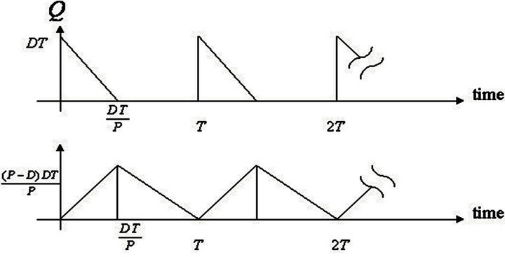
Figure 1. Inventory system for the modified EPQ model.
From the above elements, the total relevant cost per unit time can be expressed as
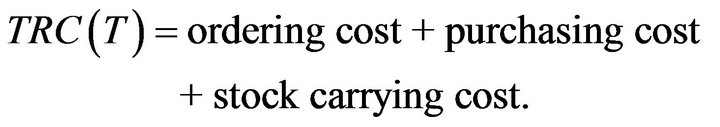
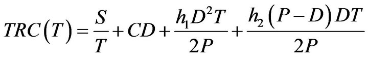 (1)
(1)
Taking the derivative of Equation (1) with respect to T
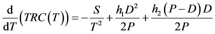 (2)
(2)
Derivative Equation (2) with respect to T,
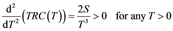 . (3)
. (3)
Equations (3) imply that  is convex on
 . We have that
  is decreasing on
  and increasing on
 .
.
Letting
 (4)
(4)
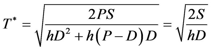
and solving Equation (4), we obtain the optimal cycle time
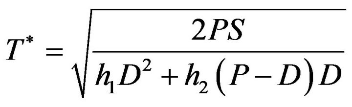 (5)
(5)
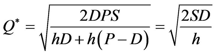
and the optimal replenishment quantity
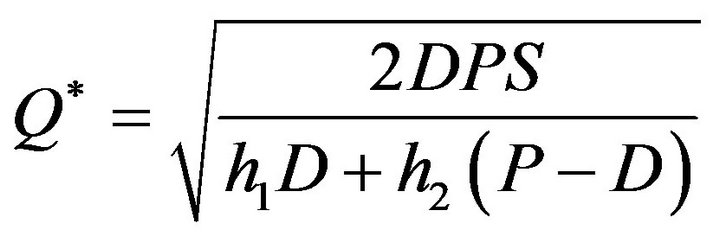 (6)
(6)
When ,
,
 (7)
(7)
 (8)
(8)
From Case 1 we can found the purchasing cost per unit time is irrelevant to time and the optimal cycle time of total relevant cost not taking the time value into consideration is the same the optimal cycle time of classical EOQ model.
Case 2. The present value of modified EPQ model.
Case 2 presents the present value for the basic EPQ model under the assumption of adding the raw materials stock-holding cost.
For this case, the stock holding cost of raw materials and products are the same. We will divide into two parts to discuss the model in the following.
(A) The present value of cash flows for the first cycle time:
First, we discuss about the inventory level of raw materials. To satisfy the demand of customers, we need to buy the amount of  in stock at the beginning of every cycle time. The level of inventory in raw materials at time
  is zero. Besides, we need to consider about the level of inventory in products. From the beginning to time
 , the products which supplier produces need to satisfy both the need of customers and accumulation of stock to sell from time to the end of cycle time
 . The annual rate of production is greater than the annual rate of demand. At time
  has the biggest amount of
  inventory in stock. Furthermore, the level of inventory of raw materials at time
  is zero. The inventory reaches the zero level at the end of the cycle time
![]() .
.
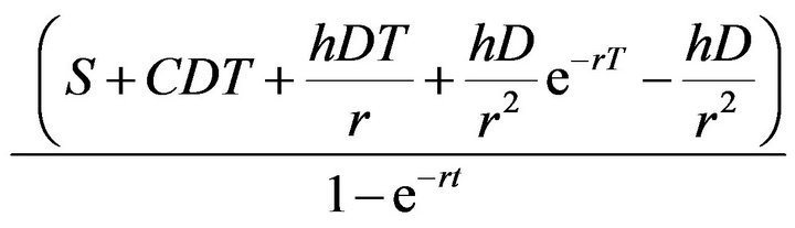
From the above arguments, we show that the present value of cash flows for the first inventory horizon,  is given by
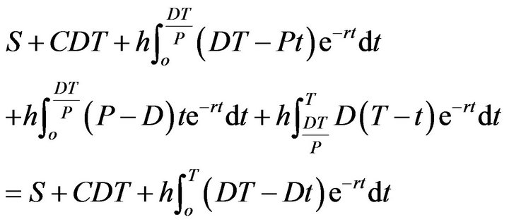 (9)
(9)
Equation (9) can be simplified as
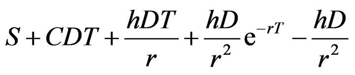 (10)
(10)
(B) The present value of cash flows for the infinite planning horizon:
If the inventory horizon from the first cycle time up to the  cycle time, then the present value is
 (11)
(11)
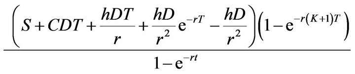
Furthermore, the present value of infinite planning horizon,  , is given by the following
 (12)
(12)
From this procedure of calculating, we found two interesting results:
1) The present value of total stock-holding cost of raw materials plus products from the beginning to time t is the same as the stock-holding cost of classical EOQ model;
2) The present value of total relevant cost is independent of the production rate (if the production rate is greater than the demand rate).
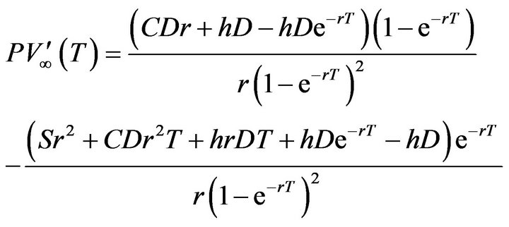
On the other hand, we can obtain an exact optimal cycle time using the following proposition and theorem.
Proposition.  has a unique local minimum on
 . Proof. Taking the first derivatives of Equation (12), is as follows
Let
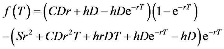 (13)
(13)
Taking the derivative of Equation (13) with respect to![]() ,
, 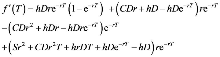
and it can be simplified as
 (14)
(14)
We have  is a strictly increasing function since
 . Since
  and
and . There exists a solution
  such that
 . Therefore,
  is a unique global minimum on
 .
.
This completes the proof.
Theorem. The upper bound of optimal cycle time is , i.e.
 .
.
Proof. From , we have
 . We known
 . (15)
Simplifying Equation (15) as follows
 (16)
(16)
and approximating  in Equation (16) by
 . Equation (16) implies that
 (17)
(17)
Considering the following equation:
 (18)
(18)
Let , then
  is the unique positive root of Equation (18). Equation (17) yields
 (19)
(19)
and  which implies that
 (20)
(20)
Combining Equation (19) and Equation (20), we obtain
 (21)
(21)
Since  is a strictly increasing function, we have
 (22)
(22)
This completes the proof.
In this case, we assume the lower bound of optimal cycle time  is zero. Combining the above theorem and proposition, we can obtain the bounds for the optimal cycle length as follows:
 (23)
(23)
In addition, we can compute an exact optimal cycle length using the logic of the following algorithm. This algorithm similar to that of Chung and Lin (cf. [7]).
The bisection algorithm ([10]):
Step 1 Let Step 2 Set
  and
and 
Step 3 Set .
.
Step 4 If , go to step 6.
Otherwise go to step 5.
Step 5 If , set
, set .
.
If , set
, set .
.
Then go to Step 3.
Step 6 . That is,
  is the exact optimal cycle length
 .
.
3. Numerical Examples
The following numerical examples are used to test and verify above theoretical results.
Example 1. Let
 ,
,  ,
,  ,
,  ,
,  ,
, .
.
Therefore,  and
and .
.
We get  and the optimal cycle length
 .
.
Example 2. Let
 ,
,  ,
,  ,
,  ,
,  ,
, .
.
Therefore,  and
and .
.
We get  and the optimal cycle length
 .
.
Example 3. Let
 ,
,  ,
,  ,
,  ,
,  ,
, .
.
Therefore,  and
and .
.
We get  and the optimal cycle length
 .
.
Example 4. Let
 ,
,  ,
,  ,
,  ,
,  ,
, .
.
Therefore,  and
and .
.
We get  and the optimal cycle length
 .
.
4. Conclusions
The classical EPQ model has been modified in order to develop a new EPQ model that can be accommodated with different situations and taking consideration of the time factor.
This study presents the modified EPQ model and the present value of cash flows for the production inventory model under the assumption of adding the raw materials holding cost. Moreover, we have shown that Case 1 and Case 2 exist an unique optimal cycle time. Numerical results of two cases are presented in Section 3. We have established the exact optimal cycle time for modified inventory model in Case 1 is larger than the present value of modified EPQ model in Case 2. This production inventory model provides an exact cycle time for many organizations. Therefore, an exact optimal cycle time can drop the total operating cost.
On the other hand, from the procedure of calculating the optimal cycle time of the total relevant cost, we found some interesting results:
1) The present value of total stock-holding cost of raw materials plus products from the beginning to time t is the same as the stock-holding cost of classical EOQ model.
2) The present value of total relevant cost is independent of the production rate (if the production rate is greater than the demand rate).
3) The optimal cycle time of total relevant cost not taking the time value into consideration is the same the optimal cycle time of classical EOQ model.
4) The purchasing cost per unit time is irrelevant to time.
REFERENCES
- E. W. Taft, “The Most Economical Production Lot,” The Iron Age, Vol. 101, 1918, pp. 1410-1412.
- I. Moon and W. Yun, “An Economic Order Quantity Model with a Random Planning Horizon,” The Engineering Economist, Vol. 39, No. 1, 1993, pp. 77-86. doi:10.1080/00137919308903113
- K. Richter, “The EOQ Repair and Waste Disposal Model with Variable Setup Numbers,” European Journal of Operational Research, Vol. 95, No. 2, 1996, pp. 313-324. doi:10.1016/0377-2217(95)00276-6
- K. J. Chung and S. D. Lin, “An Exact Solution of Cash Flow for an Integrated Evolution of Investment in Inventory and Credit,” Production Planning and Control, Vol. 9, No. 4, 1998, pp. 360-365. doi:10.1080/095372898234082
- Y. H. Kim, G. C. Philippatos and K. H. Chung, “Evaluating Investments in Inventory Systems: A Net Prexent Value Framework,” The Engineering Economist, Vol. 31, No. 2, 1986, pp. 119-136. doi:10.1080/00137918608902931
- J. T. Teng, “Discount Cash-Flow Analysis on Inventory Control under Various Supplier’s Trade Credits,” International Journal of Operations Research, Vol. 3, 2006, pp. 23-29.
- K. J. Chung and S. D. Lin, “A Note on the Optimal Cycle Length with a Random Planning Horizon,” The Engineering Economist, Vol. 40, No. 4, 1995, pp. 385-392. doi:10.1080/00137919508903162
- Y. H. Kim and K. H. Chung, “An Integrated Evolution of Investment in Inventory and Credit: A Cash Flow Approach,” Journal of Business Finance and Accounting, Vol. 17, No. 3, 1990, pp. 381-389.
- R. R. Trippi and D. E. Lewin, “A Present Value Formulation of the Classical EOQ Problem,” Decision Sciences, Vol. 5, No. 1, 1974, pp. 30-35. doi:10.1111/j.1540-5915.1974.tb00592.x
- H. E. Thompson, “Inventory Management and Captial Budgeting: A Pedagogical Note,” Decision Sciences, Vol. 6, No. 2, 1975, pp. 383-398. doi:10.1111/j.1540-5915.1975.tb01029.x
NOTES
*Corresponding author.