Engineering
Vol. 3 No. 12 (2011) , Article ID: 9205 , 10 pages DOI:10.4236/eng.2011.312145
Application of Tikhonov Regularization Technique to the Kinetic Data of an Autocatalytic Reaction: Pyrolysis of N-Eicosane
Department of Chemical Engineering, University of Lagos, Lagos, Nigeria
E-mail: *alfredasusu22@hotmail.com
Received February 12, 2011; revised March 12, 2011; accepted March 22, 2011
Keywords: Tikhonov Regularization, Thermal Decomposition, Concentration-Reaction Rate
ABSTRACT
A new technique based on Tikhonov regularization, for converting time-concentration data into concentration-reaction rate data, was applied to a novel pyrolysis investigation carried out by Susu and Kunugi [1]. The reaction which involves the thermal decomposition of n-eicosane using synthesis gas for K2CO3-catalyzed shift reaction was reported to be autocatalytic. This result was confirmed by applying Tikhonov regularization to the experimental data (conversion vs. time) presented by Susu and Kunugi [1]. Due to the ill-posed nature of the problem of obtaining reaction rates from experimental data, conventional methods will lead to noise amplification of the experimental data. Hence, Tikhonov regularization is preferably employed because it is entirely independent of reaction rate model and it also manages to keep noise amplification under control, thus, leading to more reliable results. This is shown by the agreement of the kinetic parameters obtained using the resulting conversion-reaction rate profile, with the Ostwald-type process for autocatalysis suggested by Susu and Kunugi [1].
1. Introduction
In the investigation of the kinetics of chemically reacting systems, it is often necessary to convert experimental time-concentration data into concentration-reaction rate data in order to determine the kinetic parameters of postulated reaction rate models. This has been described as an ill-posed problem in the sense that if inappropriate methods are used, the noise in the original data will be amplified leading to unreliable results. One of such procedures commonly used is that of direct numerical differentiation of the experimental data which amplifies the unavoidable noise in the experimental data [2]. Another technique attempts to integrate the rate equations in order to obtain concentration in terms of time and the unknown parameters. The unknown parameters are then determined by matching the resulting time-concentration profile with the experimental data. Unfortunately, this technique usually results in complex time-concentration profiles in which the unknown parameters are so lumped up to the extent that they cannot be determined to a reasonable degree of accuracy.
Recently, Yeow et al. [2] showed that Tikhonov regularization is a reliable procedure for converting experimental time-concentration data into concentration-reaction rate data. This procedure has been successful in keeping noise amplification under control and it also has the added advantage in that it does not require an assumed model for the reaction of interest. Having obtained the concentration-reaction rate data by Tikhonov regularization, the kinetic parameters in the rate equations are readily obtained by directly fitting these equations into the concentration-reaction rate curves. Thus, the kinetic parameters are thereby determined with relative ease and reliability.
Curve-fitting techniques are employed to estimate the kinetic parameters in the rate equations. These are numerical optimization techniques which are usually implemented by suitable commercial software such as Mathematica. The optimization technique used in the present investigation is the flexible tolerance search method of Palviani and Himmelblau [3] which was implemented by a computer programme.
In this paper, Tikhonov regularization is applied to the kinetic data reported by Susu and Kunugi [1], in which n-eicosane was thermally decomposed using synthesis gas with  -catalyzed shift reaction in a stainless steel batch reactor. Since Tikhonov regularization technique is entirely independent of reaction rate models (or reaction mechanism), it can be used as a check on the applicability of the postulated reaction mechanism for the initial decomposition reaction and the autocatalytic reaction. The experimental data of the reported pyrolysis investigation were presented in form of conversion of n-eicosane vs. time at a total initial pressure of 3.9 × 10³ kPa and at three different temperatures of 425˚C, 440˚C and 450˚C. Total n-eicosane conversion was found to be autocatalytic, a phenomenon which was attributed to the enhancement of the decomposition reaction due to the participation of allyl radicals in a new chain mechanism. Susu [4] further proposed free radical mechanism for the primary decomposition reaction and the autocatalytic reaction. The primary reaction was suggested to be first order and the activation energy of the autocatalytic reaction was found to 105
 , much lower than the activation energy of the initial decomposition reaction which would be of the order of C-C bond energy. If indeed these arguments are supported by the kinetic parameters obtained through the use of Tikhonov regularization technique, it could be used to validate the proposed reaction mechanism for the autocatalytic reaction.
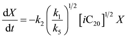
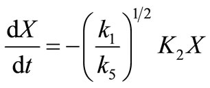
2. The Governing Equation
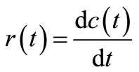
Generally, reaction rate  can be expressed in terms of concentration
  as:
as:
 (1)
(1)
which can be rewritten as:
 (2)
(2)
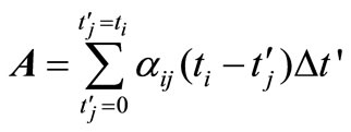
where  is the initial concentration. Equation (2) is a Volterra integral equation for the unknown reaction rate
  and initial concentration
  if this quantity is not measured directly or if the experimental measurement is considered to be unreliable. This is an integral equation of the first kind. The mathematical nature of this equation shows that the problem of obtaining
  is an illposed problem in the sense that if inappropriate methods are used, the noise in the experimentally measured timeconcentration data will be amplified leading to inaccurate results [5].
Instead of solving Equation (2) directly for , this equation, can be integrated by part as follows:
Given a function  such that
 (3)
(3)
Integrating the RHS of Equation (2) by parts gives
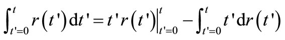 (4)
(4)
Substituting for  from Equations (3), we have
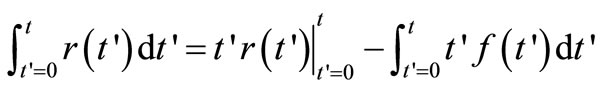 (5)
(5)
Combining Equations (2) and (5), we have
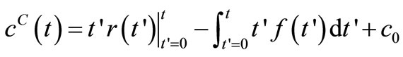 (6)
(6)
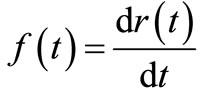
where the superscripts  and
and  are used to distinguish between the computed concentration
  and the experimentally measured concentration
 .
.
 (7)
(7)
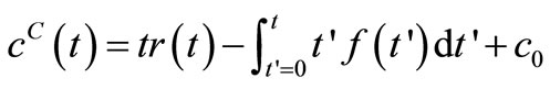
From Equation (3)
 (8)
(8)
where  is the initial rate of reaction.
Combining Equations (7) and (8), we have
 (9)
(9)
 (10)
(10)
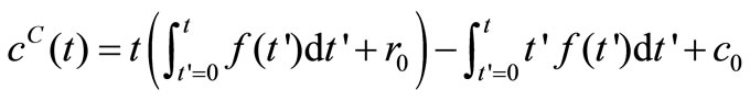
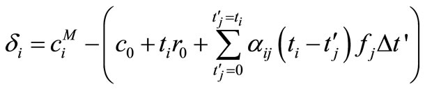
Equation (10) is the governing equation and the starting point of this investigation. It can be regarded as the Volterra integral equation of the first kind to be solved for the unknown function  and the constants
  and
and . From the way this equation was obtained it is clear that it is independent of reaction mechanism.
Given the values of ,
,  and
and ,
,  and
and  can be computed by direct numerical integ-ration. Since numerical integration does not suffer from noise amplification, the
  thus obtained is expected to be relatively free from the influence of experimental noise [2].
3. Discretization of the Volterra Integral Equation
In discretized form Equation (10) becomes
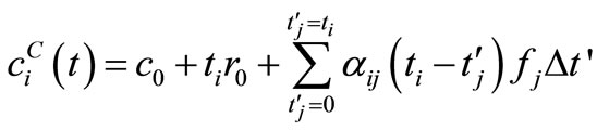 (11)
(11)
where,  , and
, and .
.
 is the number of data points, and
  is the number of discretization points.
  are the discretized
 . The independent variable
 is divided into
  uniformly spaced discretization points with step size
 , where
 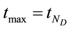 is the largest
  in the data set.
  is the coefficient arising from the numerical scheme used to approximate the integral in Equation (10). For Simpson’s
  rule, used throughout this investigation,
  for odd j (except
 ), and
  for even j.
The deviation of  from
from  is given by
 (13)
(13)
 (14)
(14)
where  and
and  and,
and,
 (15)
(15)
 (16)
(16)
 are the times at which the concentration is measured and
  are the uniformly spaced discretized time
 .
.
In matrix notation Equation (14) can be rewritten as
 (17)
(17)
where,
 (18)
(18)
 and
and  are
are  column vectors,
  is a
is a 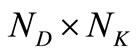 matrix of coefficient of the unknown column vector
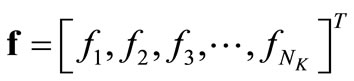 . Since
  generally exceeds the number of data points
 ,
,  is not a square matrix and Equation (14) cannot be inverted to give a unique
 ,
,  and
and . Instead, these unknowns are selected to minimize the sum of squares of
 ,
,
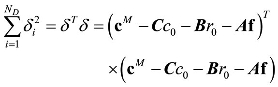 (19)
(19)
However, because of the noise in the experimental data, minimizing  will not in general result in a smooth
 . Hence, to ensure smoothness, additional conditions have to be imposed, which is the minimizetion of the sum of squares of the second derivative
 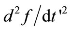 at the internal discretization points. In terms of the column vector
 , this condition takes on the form of minimizing
 (20)
(20)
where  is the tri-diagonal matrix of coefficients arising from the finite difference approximation of
  [2] and is given by
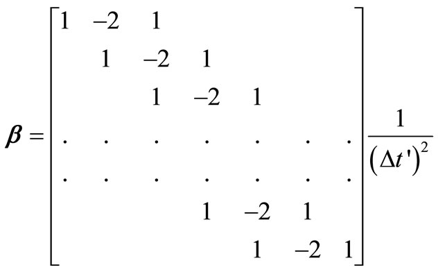 (21)
(21)
4. Tikhonov Regularization
In Tikhonov regularization [5] instead of minimizing  and
and 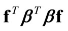 separately, a linear combination of these two quantities
 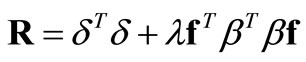 is minimized.
  is an adjustable weighting/regularization factor that controls the extent to which the noise in the kinetic data is being filtered out. Minimizing
  requires the following conditions to hold:
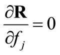 ,
,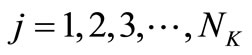 (22)
(22)
 (23)
(23)
 (24)
(24)
These give rise to a set of linear algebraic equations for ,
,  and
and  (assuming that both initial conditions are known). It can be shown [6] that the
 ,
,  and
and  that satisfy Equations (22)-(24) are given by:
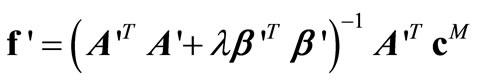 (25)
(25)
where  denotes the column vector
  incorporating
  and
and  into
into .
.  is the composite matrix
  derived from Equations (15), (16) and (18) to reflect the inclusion of
  and
and  in
in . Similarly,
  is the composite matrix
 , where
  is a
is a  column vector of 0 to allow for the fact that
  and
and  play no part in the smoothness condition in Equation (20) (Yeow et al., 2003). Equation (25) is the operating equation of Tihkonov regularization computation.
5. Implementation of the Computational Steps
The implementation of this procedure based on Tikhonov regularization involves the generation of large matrices and thus requires the use of computer programmes or suitable commercial software. In the present investigation, FORTRAN programmes were used to generate the matrices arising from Tikhonov regularization and MATLAB was used to perform the matrix operations.
Given any experimental time-concentration data, the first step is to divide the independent variable  into uniformly spaced discretization points
  with step size
 . Then, matrix
  (
( ) is determined from Equations (16) and (18) and combined with the column matrices
  and
and  to give the composite matrix
  in Equation (25). Similarly, the composite matrix
 is obtained by combining matrix
 , given by Equation (21), with the column vector
 . In order to simplify these computations, FORTRAN programmes were developed to generate matrices
  and
and  directly from experimental data. The experimental time-concentration data were inputs for these programmes and the outputs were matrices
  and
and . These matrices are usually large in size depending on the values of
  and
and . In the present investigation,
  is 6 and
  was chosen to be 21. However, larger values of
  may be used for better behaved smooth functions for
  and
and .
.
The next step is the solution of Equation (25) for values of  by simple matrix operations using MATLAB or any other commercial software. These values of
  are then substituted into the governing Equation (10) to give the concentrations
  and also into the Equation (8) to the give the reaction rates
 . Since
  is known at a large number of closely spaced discretization points, the integration for
  and
and  is carried out numerically to give well-behaved smooth functions. FORTRAN programmes were generated from Simpson’s algorithm for performing this task. The values of
  were inputs for these programmes while
  and
and  were the outputs. These computational steps are summarized in Figure 1.
6. Choice of Regularization Parameter 
The regularization parameter  is an adjustable weighting /regularization factor that controls the extent to which the noise in the kinetic data is being filtered out. It balances the two requirements on
 :
:
1) Fitting the experimental data.
2) Remaining as smooth as possible.
A large  will give a smooth
  but at the expense of the goodness of fit of the kinetic data and vice versa. The most appropriate value of
  depends on factors such as:
1) The noise level in the experimental data.
2) The number of data points .
.
3) The number of discretization points .
.
4) The numerical schemes used to approximate the integral in Equation (10) and the second derivative in Equation (20).
 is neither a property of the reaction under consideration nor a constant determined by the concentration measurement technique or instrument employed [3]. A suitable choice of the regularization parameter
  has to be provided by the user in order to apply Tikhonov regularization. In the present investigation, this choice has been guided by the simple expectation that the average and maximum deviation between
  and
and  must be physically realistic i.e. they must be comparable with the estimated magnitude of the error bars of the kinetic data while ensuring that the resulting reaction rate curve is sufficiently smooth [3]. This is otherwise referred to as the Morozov Principle [5]. This principle was applied throughout this investigation for locating the appropriate
 . The value of
  that gave the minimum deviation between
  and
and  was chosen. It was also observed that as long as
  is of the appropriate order of magnitude, changes of
  within this range do not greatly affect the final results. There are alternative methods for selecting
  such as the practical L-curve method [7] or the statistically rigorous method of Generalized Cross Validation [8].
7. Parameter Estimation and Optimization Technique
Estimating the kinetic parameters of a rate model is a very important aspect of any kinetic investigation. This can be accomplished by least-square fitting of the rate equation into the concentration-reaction rate curve. Several numerical minimization techniques have been developed to perform this task, including, simulated annealing, random search, Nelder-Mead simplex method and differentiation evolution [9]. All these minimization computations entail the assumption of initial guesses and can be performed using the commercial software Mathematica.
The general objective in optimization is to choose a set of values of variables (or parameters) subject to the various constraints that produce the desired optimum response for the chosen objective function [5]. For the flexible tolerance method [3] used in this investigation, the objective function is the sum of squares of residuals between experimental and predicted rates of reaction.
 (26)
(26)
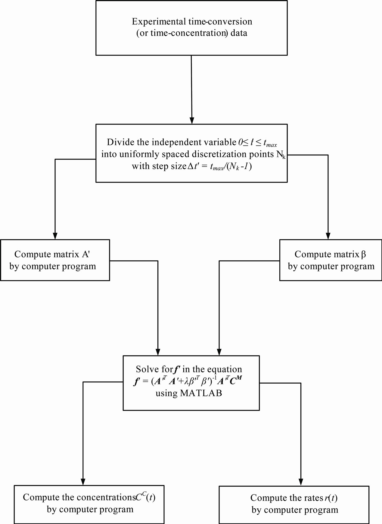
Figure 1. Schematic diagram for Tikhonov regularization solution techni-que.
The smaller the value of , the better the model and the more reliable the values of the kinetic parameters thus obtained. This method incorporates portions of the polyhedron method with the additional advantage of not restricting intermediate iteration to the feasible region. The method used here is the unweighted least square method [10] which is based on the polyhedron method of Nelder and Mead. This method alters the shape of the simplex to suit local topology. The tolerance criterion is reduced within the region of an optimum till it reaches a preset small value. This flexible tolerance method was implemented by a FORTRAN programme. The programme uses initial guesses to compute the reaction rates and then minimizes the sum of squares of errors (Equation (26)) between observed and calculated rates.
8. Reaction Mechanism and Rate Models
For the initial first-order chain sequence the following free radical mechanism was proposed for the decomposition of n-eicosane with a C-C bond scission at the  - isomer of iso-eicosane as the initiation step [4].
Initiation
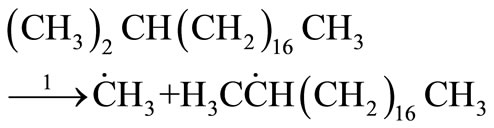 (27)
(27)
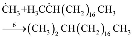
Propagation
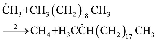 (28)
(28)
 (29)
(29)
 (30)
(30)
Termination
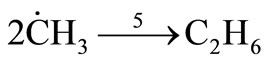 (31)
(31)
 (32)
(32)
Based on this mechanism the overall reaction rate was given as:
 (33)
(33)
This rate expression is considered as first order because the concentration of iso-eicosane  was constant throughout the decomposition reaction. The
 ’s are the rate constants in
 .
.
For the new second-order chain sequence resulting from the production of allyl radicals from propylene the following mechanism was proposed by Susu [4].
Initiation
 (34)
(34)
Propagation
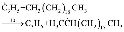 (35)
(35)
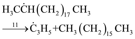 (36)
(36)
Termination
 (37)
(37)
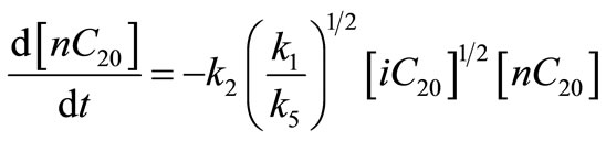
The overall rate expression for this new mechanism was given as:
 (38)
(38)
This is a second-order rate model where the ’s are the rate constants in
 . In the manner of Ostwald, the maximum rate at the inflection point was equated to
  where
where .
.  is the first-order rate constant of the decomposition reaction and
  is the bimolecular rate constant of the secondorder reaction. For autocatalysis to occur,
  and the second-order rate constant is obtained from the maximum rate. Therefore, a change in reaction rate from first to second order such that
  should explain the autocatalytic decomposition reaction in an Ostwaldtype process [11].
It is necessary to express the rate models in terms of conversion  of n-eicosane since the experimental data is presented in form of
  vs. time.
  is related to the instantaneous concentration
  and initial concentration
  by
by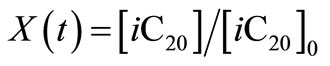 .
.
Therefore, in terms of conversion , the first-order rate expression in Equation (33) becomes
 (39)
(39)
Since 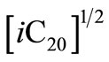 is a constant this expression can be rewritten as
 (40)
(40)
where 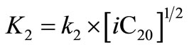 and
and ,
,  and
and  are in
 .
.
Similarly, in terms of conversion  the secondorder rate expression in Equation (38) becomes
 (41)
(41)
In this case, the data to be used for  is given in terms of moles of
  per mole of
  (dimensionless), as a result the units of
 ,
,  and
and  will be
 . These
 ’s can easily be converted into their physical equivalents in
  by dividing by the initial concentration of n-eicosane
  .
.
9. Results and Discussion
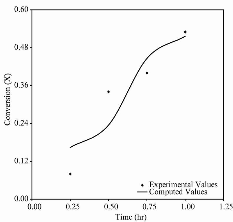
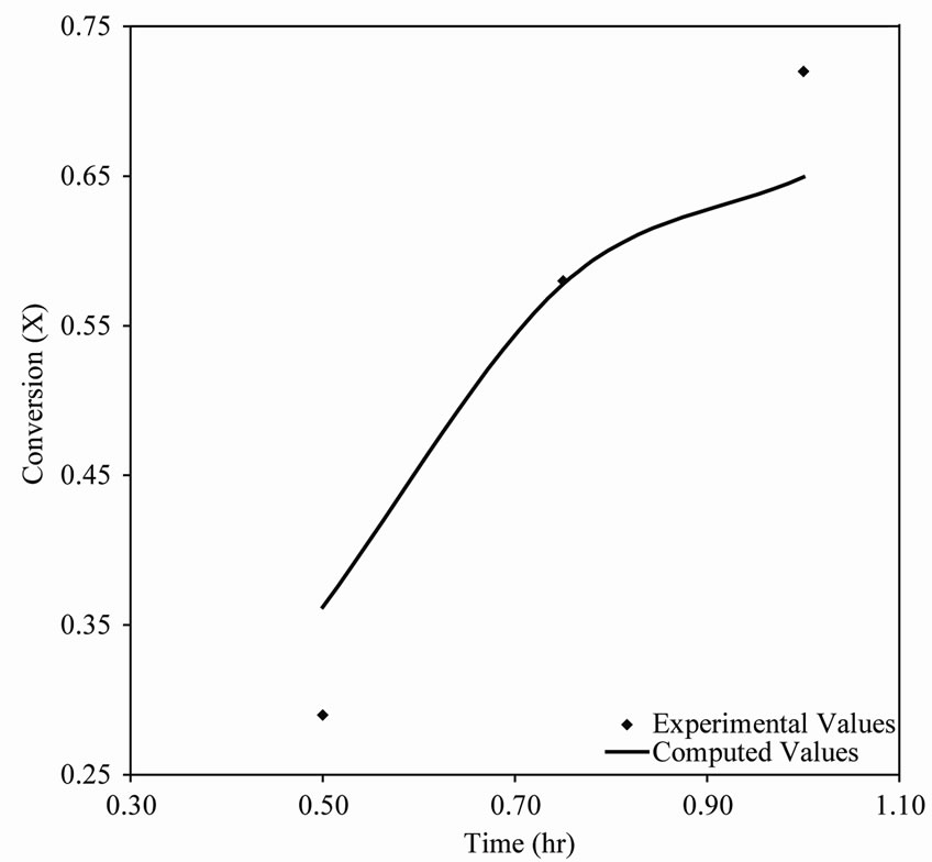
Tikhonov regularization computation has been applied to the experimental time-conversion data of the pyrolysis of n-eicosane with synthesis gas in  -catalyzed shift reaction. Susu and Kunugi [1] reported that total n-eicosane conversion was autocatalytic; a phenomenon which was attributed to the enhancement of the decomposition reaction due to the participation of allyl radicals in a new chain mechanism. For comparison, the time-conversion data obtained from Tikhonov regularization computation for
  425˚C, 440˚C and 450˚C are plotted together with the experimental data in Figures 2(a), 3(a) and 4(a) respectively. The continuous curve represents the computed conversion while the dotted curve represents the experimental data. At
  425˚C the computed conversions agree well with the experimental data and also traced out the characteristic S-shape of time-conversion curves for autocatalytic reactions [11]. At
  440˚C and
 (a)
(a)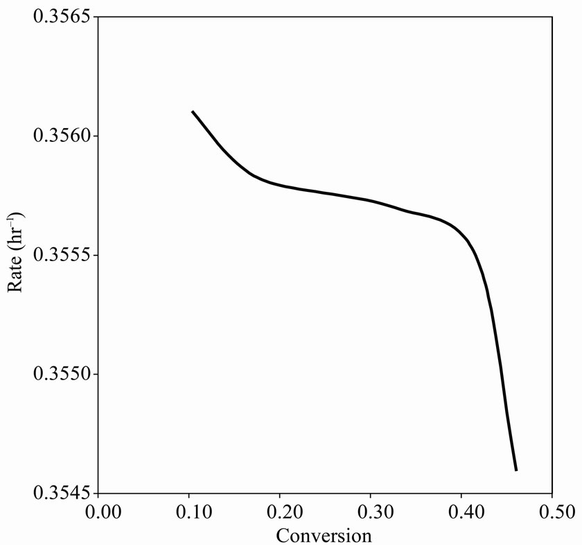 (b)
(b)
Figure 2. (a) A plot of conversion vs. time for n-eicosane pyrolysis at 425˚C. (b) Reaction rate vs. conversion curve obtained by Tikhonov regularization for n-eicosane pyrolysis at 425˚C.
 (a)
(a) (b)
(b)
Figure 3. (a) A plot of conversion vs time for n-eicosane pyrolysis at 440˚C; (b) Reaction rate vs conversion curve obtained by Tikhonov regularization for n-eicosane pyrolysis at 440˚C.
450˚C the computed conversions also agree with the experimental data but do not trace out the S-shape well enough. This resulted from the fact that the experimental data points provided at these temperatures are not sufficient (see Table 1). Thus, the experimental data for  440˚C and 450˚C were first interpolated to generate moredata points before applying Tikhonov regularization. Since interpolation will introduce some error, the conversions computed by Tikhonov regularizetion are expected to show some deviations from the original experimental data.
 (a)
(a) (b)
(b)
Figure 4. (a) A plot of conversion vs time for n-eicosane pyrolysis at 450˚C; (b) Reaction rate vs conversion curve obtained by Tikhonov regularization for n-eicosane pyrolysis at 450˚C.
Figures 2(b), 3(b) and 4(b) are plots of reaction rate vs. conversion obtained by Tikhonov regularization for  425˚C, 440˚C and 450˚C respectively. Smoothness of these curves was achieved by setting the regularizetion parameter
  to the most appropriate value which was found to be 0.015. These graphs were used to estimate the first and second order rate constants in Equations (40) and (41) respectively by least square curvefitting. As shown in Tables 2 and 3, the second-order rate constants
  are much larger than the first-order rate constants
  with
with  in the order of 10–1 to 10–2. Therefore, the values of these rate constants are in agreement with the Ostwald-type process for autocatalytic reactions (
 ) as suggested by Susu and Kunugi [1]. The plots of rate constant vs. temperature for the first and second order reaction schemes are shown in Figures 5 and 6 respectively. The rate constants increased with temperature.
The Arrhenius plots for the first and second order kinetics are shown in Figures 7 and 8, and the activation energies computed from these plots are shown in Tables 1 and 2. These activation energies are generally of the order of the C-C bond energy which agrees with that the scission of C-C bond is rate-determining in the initial decomposition reaction. Susu and Kunugi [1] reported activation energy of 105  for the bimolecular (second-order) rate constant which is also of the order of the C-C bond energy.
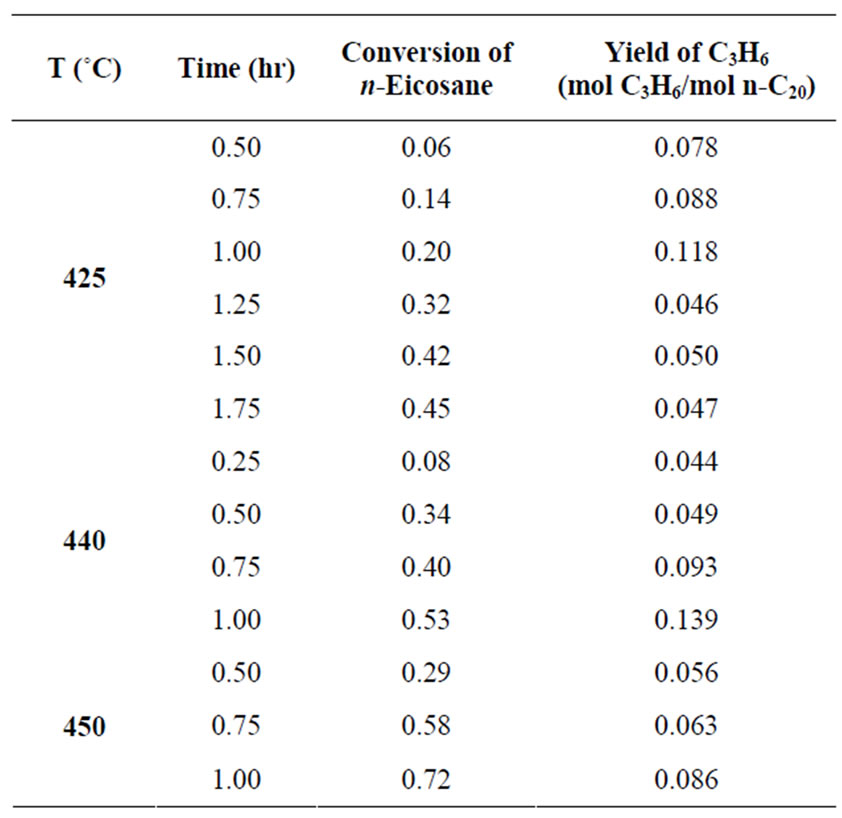
Table 1. Experimental data for the Pyrolysis of n-Eicosane.
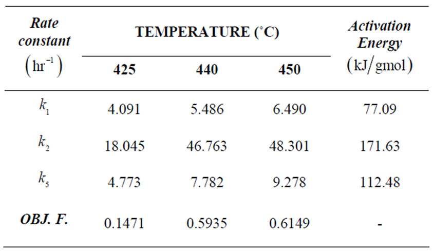
Table 2. Rate constants and objective functions for n-eicosane kinetics.
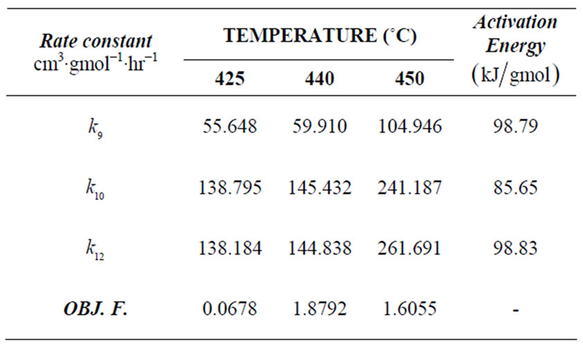
Table 3. Rate constants and objective functions for n-eicosane kinetics (Seond-order).
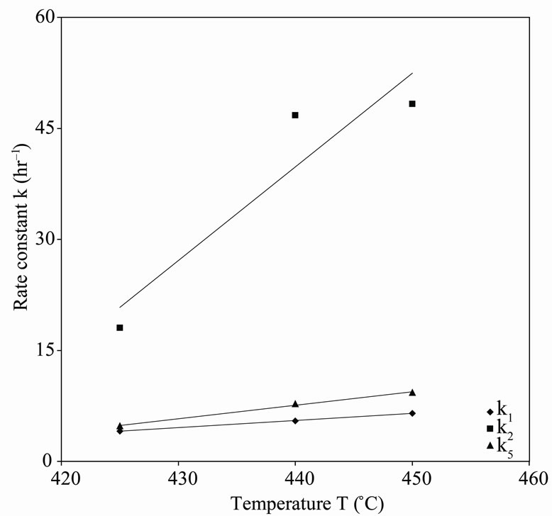
Figure 5. First-order rate constant vs. temperature for n-eicosane pyroly-sis.

Figure 6. Second-order rate constant vs. temperature for neicosane pyro-lysis.
Figure 7. Arrhenius plot for n-eicosane pyrolysis (Firstorder).
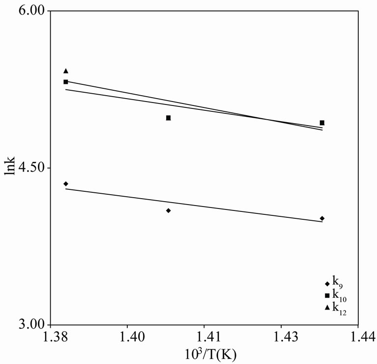
Figure 8. Arrhenius plot for n-eicosane pyrolysis (Secondorder).
10. Conclusions
Tikhonov regularization computation was successfully applied to the kinetic data of an autocatalytic reaction reported by Susu and Kunugi [1]. This method of converting time-concentration data into concentration-reaction rate data is superior to the common procedure of direct numerical differentiation of the experimental data, in the sense that it manages to keep noise amplification under control [2]. It is also independent of reaction mechanism or reaction rate model and thus provides a good check on such models accompanying any kinetic data.
In agreement with the findings of Susu and Kunugi [1], the rate constants obtained by fitting the rate equations into the conversion-reaction rate curves generated by Tikhonov regularization, were in accordance with the Ostwald-type process for autocatalysis. The values of the computed activation energies (which was in the order of the C-C bond energy) also conformed to the assumption made in the reaction mechanism that the scission of C-C bond is rate-determining in the initial decomposition reaction. Thus, these results further establish the findings of Susu and Kunugi (1980) and also show that Tikhonov regularization is a reliable technique for converting time-concentration data into concentration-reaction rate data.
11. REFERENCES
- A. A. Susu and T. Kunugi, “Novel Pyrolytic Decomposition of n-Eicosane with Synthesis Gas and
 - Catalyzed Shift Reaction,” I & EC Process Design & Development, Vol. 19, 1980, pp. 693-699.
 - Y. L. Yeow, S. R. Wickramasinghe, H. Binbing and Y. Leong, “A New Method of Processing the Time-Concentration Data of Reaction Kinetics,” Chemical Engineering Science, Vol. 58, No. 16, 2003, pp. 3601-3610. doi:10.1016/S0009-2509(03)00263-X
- G. Paviani and D. M. Himmelblau, “Constrained Nonlinear Optimization by Heuristic Programming,” Operations Research, Vol.17, No. 5, 1969, pp. 872-882. doi:10.1287/opre.17.5.872
- A. A. Susu, “Autocatalytic Decomposition of n-Eicosane in Alkali-Catalyzed
 -
- Systems,” NJET, Vol. 5, No. 1, 1982, pp. 11-19.
 - H. W. Engl, M. Hanke and A. Neubauer, “Regularization of Inverse Problems,” Kluwer Academic Publishers, Dordrecht, 1996. doi:10.1007/978-94-009-1740-8
- W. T. Shaw and J. Tigg, “Applied Mathematics: Getting Started, Getting It Done,” Addison-Wesley Publishing Co., Reading, 1994.
- P. C. Hansen, “Analysis of Discrete Ill-Posed Problems by Means of the L-Curve,” SIAM Reviews, Vol. 34, No. 4, 1992, pp. 561-580. doi:10.1137/1034115
- G. Wahba, “Spline Models for Observational Data,” CBMS- NSF Regional Conference Series in Applied Mathematics, SIAM, Philadelphia, 1990, p. 169.
- W. H. Press, S. A. Teukolsky, W. T. Vetterling and B. P. Flannery, “Numerical Recipes,” 2nd Edition, Cambridge University Press, Cambridge, 1992.
- M. Aoki, “Introduction to Optimization Techniques,” Macmillan, New York, 1971.
- M. Boudart, “Kinetics of Chemical Processes,” PrenticeHall, Englewood Cliffs, 1968.