Intelligent Control and Automation
Vol. 3 No. 1 (2012) , Article ID: 17568 , 8 pages DOI:10.4236/ica.2012.31004
Solving the Optimal Control of Linear Systems via Homotopy Perturbation Method
Department of Applied Mathematics, Ferdowsi University of Mashhad, Mashhad, Iran
Email: fatemeghomanjani@gmail.com, s_gh333@yahoo.com, farahi@math.um.ac.ir
Received November 24, 2011; revised December 22, 2011; accepted December 30, 2011
Keywords: Homotopy Perturbation Method; Optimal Control Problem; Hamilton System
ABSTRACT
In this paper, Homotopy perturbation method is used to find the approximate solution of the optimal control of linear systems. In this method the initial approximations are freely chosen, and a Homotopy is constructed with an embedding parameter , which is considered as a “small parameter”. Some examples are given in order to find the approximate solution and verify the efficiency of the proposed method.
1. Introduction
Optimal control problems arise in a wide variety of disciplines. optimal control theory has also been used with great success in areas as diverse as economics to biomedicine [1]. Apart from traditional areas such as aerospace engineering [2], robotics [3] and chemical engineering. We know that generally optimal control problems are difficult to solve. particularly, their analytical solutions are in many cases are not questionable. Thus, the key to solve many of these real world problems are numerical methods. There is a new method proposed by some authors new for solving optimal control problem based on Pontryagin’s maximum principle or Hamilton-JacobiBellman equation, such as the relaxed descent method, variation of extermal, quasilinearization, gradiant projection method [4-8]. An easy way that some author used for solving problem is to transform the problem to new problem. In [9] the problem is solved by converting the problem to differential inclusion form. In [10] the problem is converted to measure space and then solved and in [11] the problem is solved by genetic algorithm, Others deal with the optimal control problem directly. For example see [12-17].
In this paper we solve the optimal control problem by combine perturbation method. To this end, there are quite a few fundamentally diverse approaches, some of which can be found in [18,19]. The homotopy method is a powerful numerical method for solving nonlinear algebraic and functional equations. The main advantage over classical methods is that the method enjoys global convergence. However, it is not used as widely as these, mainly owing to being poorly covered in the Russian literature.
The Belgian mathematician Lahaye was the first to use the homotopy method for the numerical solution of equations. He considered the case of a single equation. He used discrete continuation by the Newton method. Later, Lahaye [20] also considered systems of equations. Davidenko [21,22] stated the method in the most effcient differential form and applied it to a wide class of problems such as the inversion of matrices, the computation of determinants, the computation of matrix eigenvalues, and the solution of integral equations. Subsequently, in [23, 24] the homotopy method was applied to boundary value problems and simplest variational problems. An essential contribution to the development of the method was made by Shalashilin, Grigolyuk, and Kuznetsov; their papers [25,26] are the most comprehensive publications on the homotopy method in Russian. The homotopy method has been developed for optimal control problems by Avvakumov [27], Since the 1980s. Allgower and Georg made an essential contribution to the popularization of the method. Their review [28] stimulated the development of the method. Of the recent publications, we note the monograph [28], where the homotopy method was combined with the Newton method or the gradient method in infinite-dimensional spaces.
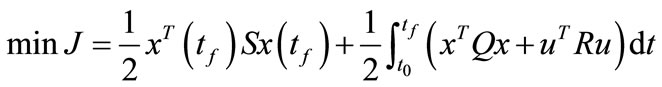
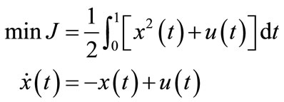
Consider the following optimal control problem

where ,
,  , and
, and ,
,  are the time invariant given matrices. The control function
  is an admissible control if it is piecewise continues in t for each t in the given interval
 . It is assumed the control is bounded, that is, a closed, bounded, subset
  of
of  exists, such that the control function takes its values form
 . The input
  can be derived by minimizing the quadratic performance index
 , where
  and
and  are symmetric positive semi-definite and
  is symmetric positive definite. By using Pontryaging’s maximum principle, the optimal control law,
  can be achieved for system (1.1) (see [34]). In this paper, we try to find an approximate value for
  by means of the perturbation homotopy method. Other numerical methods for approximating
  based on orthogonal functions are available in [29].
2. Homotopy Perturbation
Non-linear techniques for solving linear and non-linear problems have been dominated by the perturbation methods, which have found wide applications in engineering. But, like other non-linear analytical techniques, perturbation methods have their own limitations, Firstly, almost all perturbation methods are based on small parameters so that the approximate solutions can be expressed in a series of small parameters. This so called small parameter assumption greatly restricts applications of perturbation techniques, as is well known, an hefty gigantic of linear and non-linear problems have no small parameters at all. Secondly, the determination of small parameters seems to be a special art requiring special techniques. An appropriate choice of small parameters leads to ideal results, however, an unsuitable choice of small parameters results in bad effects. In 1997, Liu [30] proposed a new perturbation technique which is not based upon small parameters but upon artificial parameters, which are built in the equations.
One may consider the following nonlinear differential equation (see [31-36])
 (2.1)
(2.1)
with natural boundary conditions or tangentiality conditions as:
 (2.2)
(2.2)
where A is a general differential operator, B is a boundary operator,  is a known analytic function and
  is the boundary of the domain
 .
.
The operator  can, generally, be divided into two parts L and N, where L is Linear, while N is nonlinear, so that (2.1) may written as:
 (2.3)
(2.3)
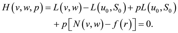
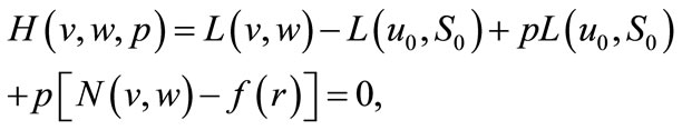
By homotopy perturbation technique, we construct a homotopy  which satisfies
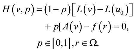 (2.4)
(2.4)
or
 (2.5)
(2.5)
where  is an embedding parameter, and
  is an initial approximate solution of Equation (2.1).
Obviously from Equation (2.5)
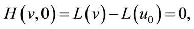 (2.6)
(2.6)
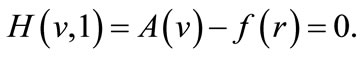 (2.7)
(2.7)
By changing continuously  from zero to unity the Equations (2.6) and (2.7) show that
  will change from
  to
to . In topology, this changing is called deformation, and
  are called homotopy functions.
In this method, using the homotopy parameter , we assume that the solution of Equation (2.5) is a power series of
 :
:
 (2.8)
(2.8)
Letting  results in the approximate solution of Equation (2.1) as:
 (2.9)
(2.9)
Series (2.9) is convergent for most cases, the convergent rate depends upon the nonlinear operator A(v).
3. Solution of the Optimal Control System
In this section, we apply the homotopy perturbation method to solve the optimal control system (1.1).
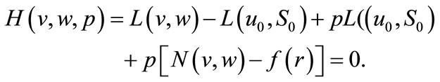
Consider Hamiltonian of the control system (1.1) as:
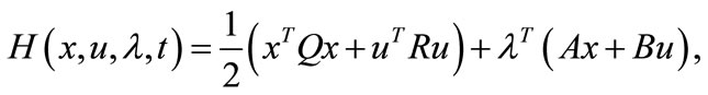 (3.1)
(3.1)
where  is known as the costate variable. By Pontryagin’s maximum principle, the optimal control must satisfy the following equation:
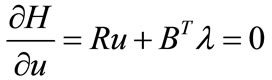 (3.2)
(3.2)
where  is a solution of the adjoint equation
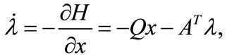 (3.3)
(3.3)
with the terminal condition
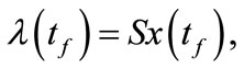 (3.4)
(3.4)
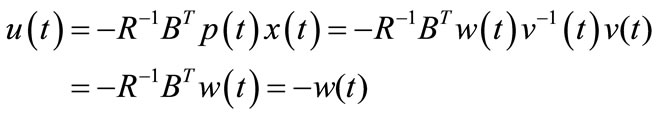
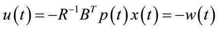
Thus, from Equation (3.2), the optimal control law is
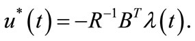 (3.5)
(3.5)
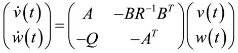
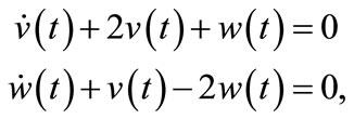
From control system (1.1) and adjoint Equation (3.3) one have:
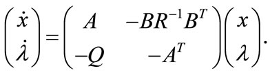 (3.6)
(3.6)
Implementing the optimal control as a closed loop if the solution to the adjoint Equation (3.3) is assumed like Equation (3.4) as a linear function of the states in the form( see [29]),
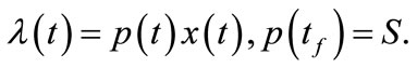 (3.7)
(3.7)
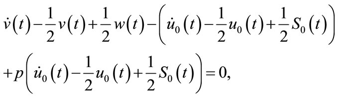
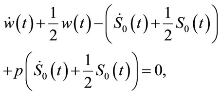
By using Equations (3.3), (3.6) and (3.7), we have
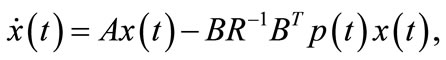

where the first equality follows from Equation (3.7) and the second one from Equation (3.6). Hence
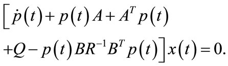 (3.8)
(3.8)
Since the above equation must hold for all nonzero ,
,  must satisfy the following matrix Riccati equation
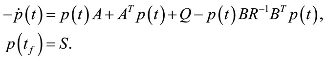 (3.9)
(3.9)
Considering Equations (3.5) and (3.7), we can see that the optimal control law is given as
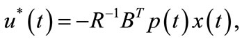 (3.10)
and  can be computed using the following relation
 (3.11)
where ,
, 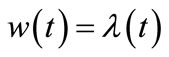 and
and
with conditions, 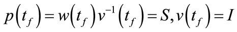 and
and 
4. Numerical Examples
In this section, we present some examples to show the reliability and efficiency of the method described in the previous section. In the following examples, we assume .
.
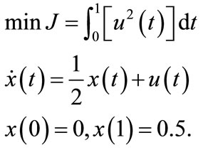
Example 4.1. Consider a single-input scalar system as follows (see [29]):
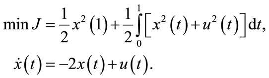
According to system (1.1), we have 
 and
and  by using (3.12), we have
thus
So

by using (2.8), let  and
and  so,
so,
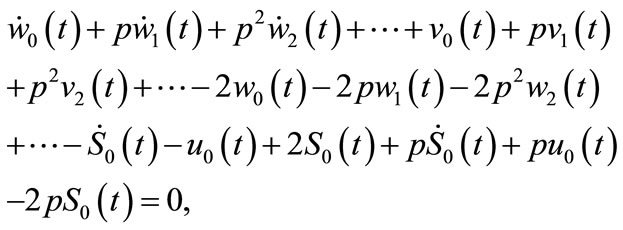
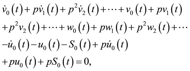
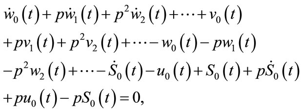
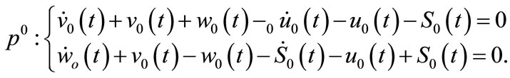
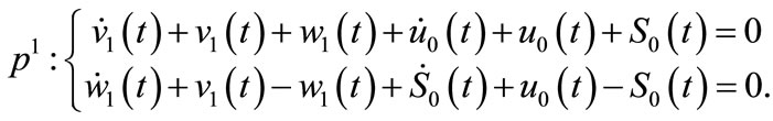
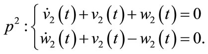
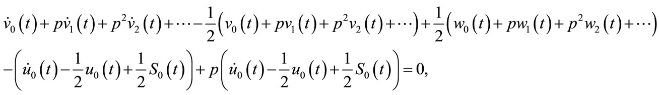
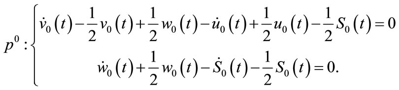
from equating the terms with identical power of p,
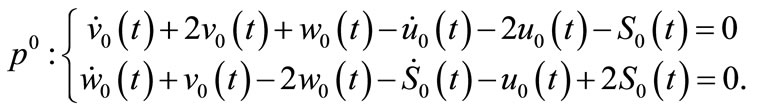 (4.1)
(4.1)
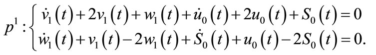 (4.2)
(4.2)
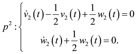
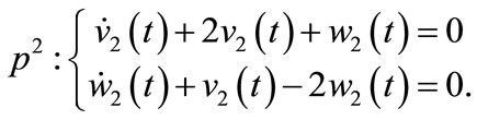 (4.3)
(4.3)
where 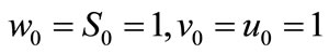 are considered as initial approximations, and imposing boundary condition, so
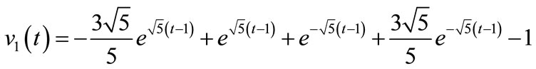
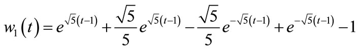
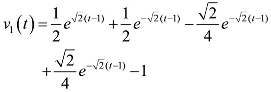
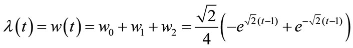
by using (4.3), we have

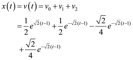
From (2.9), we have
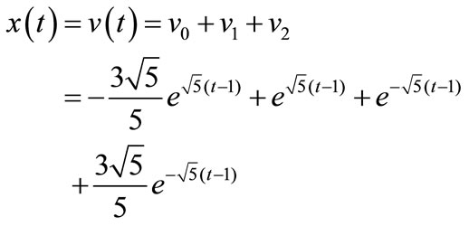
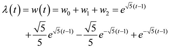
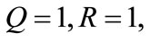
Figures 1 and 2 show the approximated value of  and
and , respectively.
Example 4.2. Consider a single-input scalar system as follows (see [29]):
According to system (1.1), we have 
 and
and , by using (3.12), we have
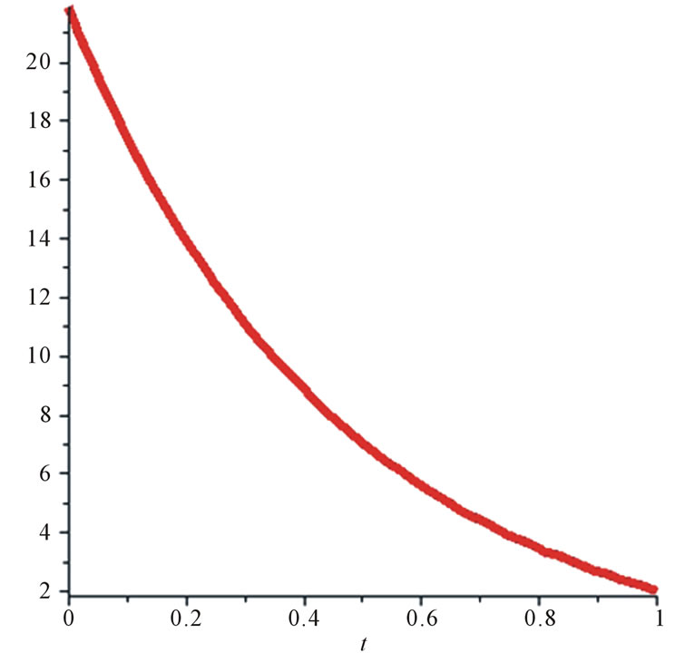
Figure 1. Approximate state x(t) for Example 4.1.
Figure 2. Approximate control u(t) for Example 4.1.
thus
So

by using (2.8), we have
from equating the terms with identical power of p,
where  are considered as initial approximations, Setting
  and imposing boundary condition, so

by using (4.3), we have
From (2.9), we have
 .
.
Figures 3 and 4 show the approximated value of x(t) and u(t), respectively.
Example 4.3. Consider a single-input scalar system as follows:
According to system (1.1), we have 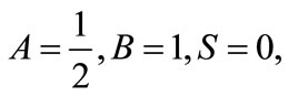
 and
and  and by using (3.12), we have
thus
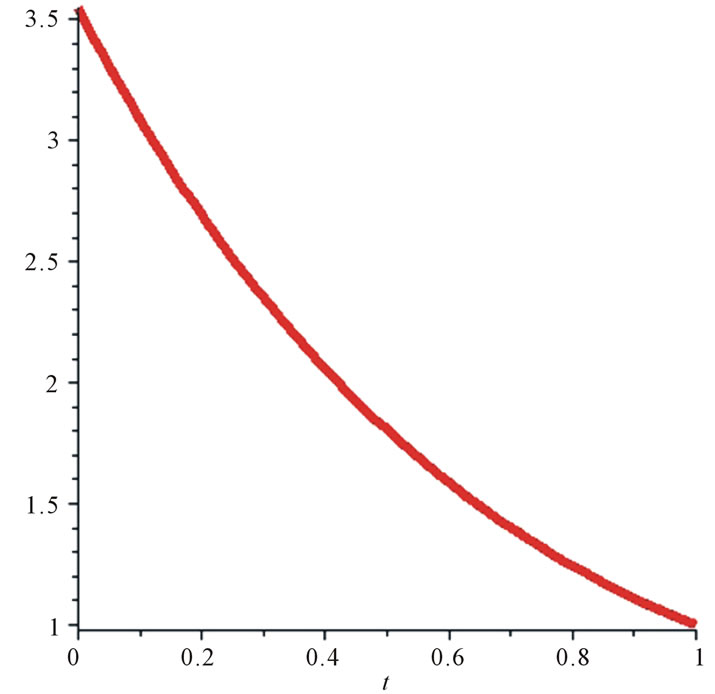
Figure 3. Approximate state x(t) for Example 4.2.
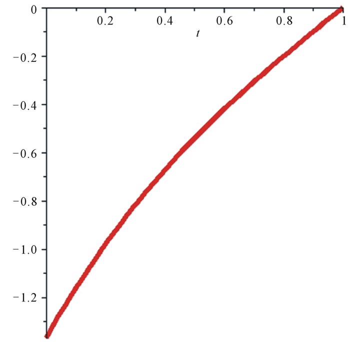
Figure 4. Approximate control u(t) for Example 4.2.
So
by using (2.8), we have

from equating the terms with identical power of p,

where, 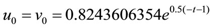 are considered as initial approximations, Setting
  and imposing boundary condition, the approximate and exact value for
  is
is 
 the
the
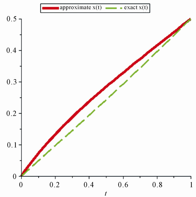
Figure 5. Approximate and exact solution x(t) for Example 4.3.
exact value for  is
is  and the approximate value for
  and
and  obtained from this algorithm in this following form
Figure 5 compares the exact and approximate solution of x(t), and Figure 6 shows the residual function.
5. Conclusions
In this paper, we solve the optimal control problems us-
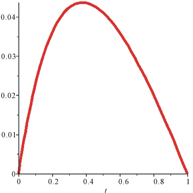
Figure 6. Residual function for Example 4.3.
ing Homotopy perturbation method. Embedding parameter  can be taken into account as a perturbation parameter. Full advantage of the traditional perturbation techniques can be taken by the novel method. The initial approximation can be freely chosen with unknown constants, which can be identified via various methods [35].
At last, Homotopy perturbation method is applicable method which calculates the approximate solution of linear and nonlinear problems, particularly optimal control problems.
REFERENCES
- M. Itik, M. U. Salamci and S. P. Banksa, “Optimal Control of Drug Therapy in Cancer Treatment,” Nonlinear Analysis, Vol. 71, No. 12, 2009, pp. e1473-e1486. doi:10.1016/j.na.2009.01.214
- W. L. Garrard and J. M. Jordan, “Design of Nonlinear Automatic Flight Control Systems,” Automatic, Vol. 13, No. 5, 1977, pp. 497-505. doi:10.1016/0005-1098(77)90070-X
- S. Wei, M. Zefran and R. A. DeCarlo, “Optimal Control of Robotic System with Logical Constraints: Application to UAV Path Planning,” Proceedings of the IEEE International Conference on Robotic and Automation, Pasadena, 19-23 May 2008, pp. 176-181.
- I. Chryssoverghi, J. Coletsos and B. Kokkinis, “Approximate Relaxed Descent Method for Optimal Control Problems,” Control and Cybernetics, Vol. 30, No. 4, 2001, pp. 385-404.
- D. E. Kirk, “Optimal Control Theory: An Introduction,” Prentice-Hall, Upper Saddle River, 1970.
- J. C. Dunn, “On L2 Sufficient Conditions and the Gradient Projection Method for Optimal Control Problems,” SIAM Journal of Continues Optimal, Vol. 34, No. 4, 1996, pp. 1270-1290. doi:10.1137/S0363012994266127
- R. W. Beard, G. N. Saridis and J. T. Wen, “Approximate Solutions to the Time-Invariant Hamilton-Jacobi-Bellman Equation,” Optimal Theory Application, Vol. 96, No. 3, 1998, pp. 589-626. doi:10.1023/A:1022664528457
- I. Chryssoverghi, I. Coletsos and B. Kokkinis, “Discretization Methods for Optimal Control Problems with State Constraints,” Journal of Computational and Applied Mathematics, Vol. 19, No. 1, 2006, pp. 1-31. doi:10.1016/j.cam.2005.04.020
- A. V. Kamyad, M. Keyanpour and M. H. Farahi, “A New Approach for Solving of Optimal Nonlinear Control Problems,” Applied Mathematics. Computers, Vol. 187, No. 2, 2007, pp. 1461-1471. doi:10.1016/j.amc.2006.09.051
- S. Effati, M. Janfada and M. Esmaeili, “Solving the Optimal Control Problem of the Parabolic PDEs in Exploitation of Oil,” Journal of Mathematical Analysis and Applications, Vol. 340, No. 1, 2008, pp. 606-620. doi:10.1016/j.jmaa.2007.08.037
- O. S. Fard and H. A. Borzabadi, “Optimal Control Problem, Quasi-Assignment Problem and Genetic Algorithm,” Proceedings of World Academy of Science, Engineering and Technology, Vol. 21, 2007, pp. 70-43.
- K. L. Teo, C. J. Goh and K. H. Wong, “A Unified Computational Approach to Optimal Control Problem,” Longman Scientific and Technical, Harlow, 1991.
- H. Hashemi Mehne and A. Hashemi Borzabadi, “A Numerical Method for Solving Optimal Control Problem Using State Parametrization,” Numerical Algorithms, Vol. 42, No. 2, 2006, pp. 165-169. doi:10.1007/s11075-006-9035-5
- G. N. Elnagar, “State-Control Spectral Chebyshev Parameterization for Linearly Constrained Quadratic Optimal Control Problems,” Computational Applied Mathematics, Vol. 79, No. 1, 1997, pp. 19-40. doi:10.1016/S0377-0427(96)00134-3
- J. Vlassenbroeck and R. V. Dooren, “A Chebyshev Technique for Solving Nonlinear Optimal Control Problems,” IEEE Transactions on Automatic Control, Vol. 33, No. 4, 1998, pp. 333-340. doi:10.1109/9.192187
- H. R. Sirsena and K. S. Tan, “Computation of Constrained Optimal Controls Using Parameterization Techniques,” IEEE Transactions on Automatic Control, Vol. 19, No. 4, 1974, pp. 431-433.
- H. P. Hua, “Numerical Solution of Optimal Control Problems,” Optimal Control Applications and Methods, Vol. 21, No. 5, 2000, pp. 233-241. doi:10.1002/1099-1514(200009/10)21:5<233::AID-OCA667>3.0.CO;2-B
- V. V. Dikusar, M. Kosh’ka and A. Figura, “Parametric Continuation Method for Boundary-Value Problems in Optimal Control,” Differentsial/cprime nye Uravneniya, Vol. 37, No. 4, 2001, pp. 453-457.
- M. Weiser, “Function Space Complementarity Methods for Optimal Control Problems,” Dissertation Eingereicht am Fachbereich Mathematik und Informatik der Freien Universitat, Berlin, 2001.
- M. E. Lahaye, “Solution of System of Transcendental Equations,” Académie Royale de Belgique. Bulletin de la Classe des Sciences, Vol. 5, 1948, pp. 805-822.
- D. F. Davidenko, “Solution of System of Transcendental Equations,” Dokl. Akad. Nauk, Vol. 88, No. 4, 1953, pp. 601-602.
- D. F. Davidenko, “Approximate Solution of Systems of Nonlinear Equations,” Ukr. Mat. Zh., Vol. 5, No. 2, 1953, pp. 196-206.
- V. E. Shamanskii, “Metody Chislennogo Resheniya Kraevykh Zadach na EtsVM (Numerical Methods for the Solution of Boundary Value Problems on Computer),” Naukova Dumka, Kiev, 1966.
- S. Roberts and J. S. Shipman, “Continuation in Shooting Methods for Two-Point Boundary Value Problems,” Journal of Mathematical Analysis and Applications, Vol. 18, No. 1, 1967, pp. 45-58. doi:10.1016/0022-247X(67)90181-3
- E. I. Grigolyuk and V. I. Shalashilin, “Problemy Nelineinogo Deformirovaniya (Problems of Nonlinear Deformation), Nauka, Moscow, 1988.
- V. I. Shalashilin and E. B. Kuznetsov, “Metod Prodolzhneiya Resheniya po Parametru i Nailuchshaya Parametrizatsiya (The Homotopy Method of Continuation and Best Parametrization),” Editorial URSS, Moscow, 1999.
- S. N. Avvakumov, “Smooth Approximation of Convex Compacta,” Trudy Instituta. Matematiki. i Mekhaniki. UrO RAN, Ekaterinburg, Vol. 4, 1996, pp. 184-200.
- E. L. Allgower and K. Georg, “Introduction to Numerical Continuation Methods,” SIAM, Berlin, 1990.
- S. A. Yousefi, M. Dehghan and A. Lotfi, “Finding Optimal Control of Linear Systems via He’s Variational Iteration Method,” Computational Mathematics, Vol. 87, No. 5, 2010, pp. 1042-1050.
- G. L. Liu, “New Research Directions in Singular Perturbation Theory: Artificial Parameter Approach and Inverse Perturbation Technique,” Proceeding of the 7th Conference of the Modern Mathematics and Mechanics, Shanghai, September 1997, pp. 47-53.
- S. Abbasbandy, “Homotopy Perturbation Method for Quadratic Riccati Differential Equation and Comparision with Adomian’s Decomposition Method,” Applied Applied Mathematics and Computation, Vol. 172, 2006, pp. 482-490.
- D. Ganji, H. Tari and M. Bakhshi, “Variational Iteration Method and Homotopy Perturbation Method for Nonlinear Evalution Equations,” Computers & Mathematics with Applications, Vol. 54, No. 7-8, 2007, pp. 1018-1024. doi:10.1016/j.camwa.2006.12.070
- J.-H. He, “A Coupling Method for a Homotopy Technique and a Perturbation Technique for Nonlinear Problems,” International Journal of Non-Linear Mechanics, Vol. 35, No. 1, 2000, pp. 37-43.
- J.-H. He, “Homotopy Perturbation Method: A New Nonlinear Analytical Technique,” Applied Mathematics and Computation, Vol. 135, No. 1, 2003, pp. 73-79. doi:10.1016/S0096-3003(01)00312-5
- J.-H. He, “Homotopy Perturbation Method for Solving Boundary Value Problems,” Physics Letters A, Vol. 350, No. 1-2, 2006, pp. 87-88. doi:10.1016/j.physleta.2005.10.005
- J.-H. He, “Homotopy Perturbation Technique,” Applied Mathematics and Computation, Vol. 178, No. 2, 1997, pp. 257-262.