Materials Sciences and Applications
Vol.10 No.06(2019), Article ID:93171,21 pages
10.4236/msa.2019.106035
Crack Prediction Model for Concrete Affected by Reinforcement Corrosion
Jeb M. Stefan1, Luz M. Calle2, Sven E. Eklund3, Mark R. Kolody2, Kunal Kupwade-Patil4, Eliza L. Montgomery2, Henry E. Cardenas3
1University of Texas in Austin, Austin, USA
2NASA, John F. Kennedy Space Center, Kennedy Space Center, Merritt Island, USA
3Louisiana Tech University, Ruston, USA
4Department of Civil and Environmental Engineering, Massachusetts Institute of Technology, Cambridge, USA

Copyright © 2019 by author(s) and Scientific Research Publishing Inc.
This work is licensed under the Creative Commons Attribution International License (CC BY 4.0).
http://creativecommons.org/licenses/by/4.0/


Received: March 6, 2019; Accepted: June 21, 2019; Published: June 24, 2019
ABSTRACT
The purpose of this study was to develop an analytical model to predict the time required for cracking of concrete due to corrosion of the iron reinforcement. The concrete and cement specimens used for this study were batched with cover material ranging from 0.75 to 1.3 in (1.91 to 3.30 cm). The extent of cover material was not formulated into the model under the assumption that crack initiation would tend to produce visible cracking within a relatively short time period. The model was derived using both Hooke’s Law and the volume expansion induced by the corrosion oxides. Correlation achieved with specimen cracking data from the literature was relatively good with a 95% level of confidence. This model presents a key benefit to facility and infrastructure managers by enabling them to plan the time when corrosion mitigating actions are required. It also provides a significant convenience as the condition of the concrete structure or its environment changes over time. The only parameter that needs to be updated over time is the corrosion rate measurement. This single parameter captures the most influential impact that stems from several other parameters which tend to be required in models that are more mechanistically definitive.
Keywords:
Cracking, Model, Concrete, Corrosion, Marine, Pore Band, Green Rust

1. Introduction
Aggressive chemical species can migrate through the pore structure of concrete and cause corrosion of the embedded steel reinforcement. Corrosion reactions taking place on the surface of the reinforcement tend to convert the iron into various oxides. These corrosion products are less dense and occupy considerably more space than the original reinforcement, increasing the overall volume occupied by the reinforcement. This results in a tensile stress on the surrounding concrete which leads to cracking and structural failure.
Corrosion of the reinforcement occurs due to the electrochemical cells produced by a drop in pH or the exposure to chlorides and sulfides [1] [2] . The corrosive anions are either transported from the outside environment or they are leached from contaminated aggregate within the concrete [3] [4] . The corrosion of the reinforcement compromises the overall structure as the cross-sectional area of the original reinforcement material is oxidized and replaced by weaker and more brittle corrosion products. The allowable loading of the remaining metal will fall below that of the original design for the structure. Another compromising problem associated with the corrosion of the reinforcement is that as corrosion products are formed on the surface of the reinforcement, there is an expansion of the area occupied by the reinforcement and its oxides. This enlarging cross-sectional area produces a tensile stress in the surrounding concrete. Although concrete is strong in compression, it is unfortunately weak in tension. The objective of this work was to develop an analytical model for predicting the amount of time before a crack would be formed in concrete due to the corrosion of the embedded reinforcement.
2. Research Significance
Concrete cracking due to the corrosion of the reinforcement incurs significant costs to the public and private sector. The repair of reinforced concrete is costing over $20 billion/year in the US just in the transportation infrastructure alone [5] . A simple analytical model for predicting the time before crack initiation in reinforced concrete due to reinforcement corrosion would enable better design and maintenance management of our infrastructure assets.
3. Experimental Procedure
The experimental work in this study focused on characterizing the mechanisms, kinetics, and speciation of reinforcement corrosion with in calciumaluminate cement (CAC) and Type I Portland cement (OPC) concrete. The data from this work was used to develop a model for determining cracking time of the cover material due to the corrosion of the reinforcement. Data collected for this study was obtained at Louisiana Tech University and NASA’s John F. Kennedy Space Center (KSC) from 2008-2015.
For the OPC concrete specimens, Type I Portland cement was used. Water, sand, and Arkansas pea gravel were added to the cement powder to form mixes batched at mass ratios of 0.5, 2.6, and 1.5 with respect to the cement powder in accordance with ASTM C192 [6] and ASTM C195 [7] . Each cylindrical specimen contained a 1018 steel rod as reinforcement that was 0.25 in (0.635 cm) in diameter with 1.3 in (3.3 cm) of concrete cover. The overall concrete specimen diameter was 2.875 in (7.30 cm) and the height was 6 in (15.24 cm). The 1018 steel had an iron content of over 98% [8] . The CAC specimens were batched from a Fondu Fyre cement paste (obtained from Pryor Giggey Co., Anniston, AL). It was a proprietary formulation that was mixed with water per the supplier’s instructions. The porosity was increased by using additional water (+15% by mass) to provide for rapid flash steam resistance associated with rocket launches. ASTM C862 [9] was followed for all of the CAC specimen batch processes. Control specimens were batched with freshwater while companions were batched with 4.5 wt% salt water. A vibration table was used to mitigate void formation. The cylindrical CAC specimens contained the same diameter of 1018 steel rod embedded with 0.75 in (1.91 cm) of cover material. The overall specimen diameter was 1.75 in (4.45 cm) while the height was 3.875 in (9.84 cm). Both specimen types were placed in the salt water immersion tank located at the Kennedy Space Center (KSC) Beachside Atmospheric Corrosion Test Site in Kennedy Space Center, FL. This tank received sea-water that was pumped 300 ft (91 m) from the Atlantic Ocean. The water was obtained from just below the low tide line [10] . Water temperatures during a 6-year exposure period fluctuated between 68˚F (20˚C) to 82.4˚F (28˚C) over the course of daily and seasonal cycles. A salt spray system located above the specimens provided additional oxygenation of the tank water.
While undergoing salt water exposure at KSC both types of specimens were subjected to potentiostatic corrosion rate measurements using a copper-copper sulfate (Cu/CuSO4) reference electrode and a graphite counter electrode. Corrosion rate measurements at KSC were conducted at the laboratory at the KSC Beachside Atmospheric Corrosion Test Site using a Gamry Instruments Reference 600 potentiost (manufactured in Warminster, PA). Corrosion rate measurements conducted at Louisiana Tech University utilized a Solartron SI 1287 potentiost at (manufactured by Ametek Inc. in Oak Ridge, TN). A Stern-Geary coefficient of 68 mV was recommended by Jones to account for submersion of steel in 3.5 wt% salt water [11] . CorrView software (produced by CorrView LLC, in Landing, NJ) was used to run the potentiostatic measurements. A plot of current versus potential was generated. The slope of potential versus current density at the origin of this plot is known as the polarization resistance (Rp). This can be related to the Stern-Geary relationship to find the corrosion current density (Icorr) [11] [12] . The corrosion current density was used to calculate the corrosion rates [13] . The IR drop was corrected using a feedback compensation technique.
The porosity of both the cement and concrete specimens was evaluated via water mass loss that was induced by heating at 105˚C (221˚F). The amount of imbibed water present in the corrosion products was determined immediately following in-direct tensile testing. As per the porosity testing, these oxide samples were heated to 105˚C (221˚F) in order to drive off the imbibed water. Raman Spectroscopy and Energy Dispersive Spectroscopy (EDS) were conducted to identify corrosion products present at the time of specimen tensile testing and after lab-atmosphere exposure was permitted to chemically alter these oxides. This information was used later to interpret the data obtained from the imbibed water assessment which also involved atmospheric exposure. Additional analysis included scanning electron microscopy (SEM). These characterization tools made it possible to de-convolute the mass loss of imbibed water from the mass gain of corrosion product oxidation that occurred during sample heating. The microscopy and EDS work was conducted using a field emission scanning electron microscope (FESEM), the Hitachi S4800 SEM (manufactured by Hitachi Ltd. of Tokyo, Japan), in coordination with an EDAX Genesis XM-4 analyzer (manufactured by Ametek Inc. in Mahwah, NJ). An Xplora Plus Raman microscope (manufactured by Horiba Scientific, Japan) was also used to investigate oxide phases in this study. The 532 nm green laser was used after it was determined that the 785 nm red laser produced significant background fluorescence.
4. Experimental Results
The analytical model required information regarding the reinforcement corrosion rate, volume expansion and transport characteristics of the corrosion products, and the porosity of the concrete cover. The following sections contain the results of work conducted to acquire useful values for these model parameters.
4.1. Specimen Corrosion Rate Measurements
Corrosion rates of specimens were obtained relatively early in the exposure period as well as shortly before destructive testing (See Table 1). Corrosion rate data was also recorded for companion specimens that were exposed only to atmospheric exposure at the same beachside location adjacent to the seawater immersion tank. As expected, the waterline immersion specimens corroded at a faster rate than the atmospheric exposure controls.
The corrosion rate of the reinforcement is generally highest when the surface of the material is not covered with corrosion products [3] . As the corrosion

Table 1. Corrosion rate data for specimens.
*Corrosion rates from the early exposure period (<3 yr) were taken at KSC while all data from the extended exposure period (>5 yr) was taken after the transfer of the specimens to Louisiana Tech University.
products build up on the surface, the rate of deterioration of the original reinforcement will decrease as resistance induced by the oxide layer increases over time. After an extended period of time, the corrosion rate is generally expected to be relatively steady or slowly declining at a rate which is dependent upon the chemistry of the environment, the resistance of the corrosive medium, and the chemistry of the corroding material [11] . The corrosion rates for specimens which have been corroding for over five years, shown in Table 1, exhibited this type of behavior. The average specimen corrosion rate for the group of six Type I OPC concrete specimens after five years of exposure was 0.84 mpy (0.02 mm/yr) while the group of six CAC specimens exhibited an average corrosion rate of 1.12 mpy (0.03 mm/yr). This data was useful because it confirmed that these specimens were corroding at reasonable and declining rates for an extended water-line exposure period in the sea-water environment [14] .
4.2. Porosity Measurements
The porosity of several specimens was measured in order to characterize the available space into which corrosion products could escape from the reinforcement via diffusion. These migrated products no longer remained on the bars where they could contribute to tensile stress development. This migration of corrosion products was a key consideration in the formulation of the crack initiation time model. Both of the concrete specimen types exhibited porosities of approximately 7% (the CAC specimens had porosities of 7% ± 3% and the Type I OPC concrete specimens exhibited porosities of 7.6% ± 0.3%). The confidence interval for these results was 90%.
These measurements were clearly reproducible as indicated by the relatively small scatter observed in the porosity data. In general, the relatively low level of porosity observed may stem from the several desiccation periods that occurred while in the seawater immersion tank at KSC. The exposure history included periodic maintenance interruptions. A drop in pore size could be anticipated due to capillary forces that cause drying shrinkage of the surrounding material matrix [14] .
4.3. Corrosion Product Observations
Specimens that were broken for examination of the embedded reinforcement clearly exhibited several corrosion product stoichiometries based on the multiple colors visually observed [15] . The primary iron oxide color observed was green. Figure 1 shows the location of the rebar on a fracture surface of a Type I OPC specimen and the extent to which the oxide penetrated into the surrounding concrete [14] .
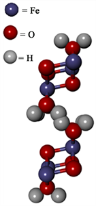
The presence of the green corrosion products, along with the exposure to a chloride-rich, aqueous corrosion environment, suggests that the product formed was “green rust,” commonly denoted as GR1(Cl−) with the stoichiometry FeII3FeIII(OH)8Cl−. Raman spectroscopic analysis was conducted to examine the stoichiometry of these corrosion products. Figure 2(a) displays the Raman spectrum of a green corrosion product sample obtained from a CAC specimen that was permitted to oxidize after exposure to laboratory air. Figure 2(b) represents the unit cell of lepidocrocite (γ-FeO(OH)).
The most common Raman peaks associated with green rust (FeII3FeIII(OH)8Cl−) are 427 and 518 cm−1 [16] . The bands shown in Figure 2(a) were typical of those observed in the Raman spectra recorded for several sampling locations. These peaks were in the vicinity of 217, 276, and 378 cm−1. None of these peaks were indicative of green rust. As explained in the literature, green rust is formed in the absence of oxygen and will rapidly transform into other iron oxide phases upon exposure to air [16] [17] . In the current study, these samples were given the opportunity to transform prior to the Raman analysis (This information was

Figure 1. Presence of corrosion oxides on the fracture surface of a Type I OPC concrete specimen photographed following in-direct tensile testing. The darkest areas were locations of green oxide. This specimen was subjected to approximately six years of water-line exposure in the seawater immersion tank at the KSC Beachside Atmospheric Corrosion Test Site in Kennedy Space Center, FL.
 (a)
(a)
 (b)
(b)
Figure 2. (a) Raman spectrum from green rust location on reinforcement. This CAC specimen was permitted to oxidize in laboratory air prior to obtaining the spectrum. This spectrum facilitated the interpretation of the results of the imbibed water tests that were utilized in the cracking model; (b) Unit cell of lepidocrocite.
useful for interpreting the analysis of imbibed water). Some peaks typically associated with lepidocrocite were visible in Figure 2(a) and unit cell of this corrosion product is shown in Figure 2(b). Lepidocrocite is characterized by a strong peak around 250 cm−1, two medium peaks at 379 and 528 cm−1 , and smaller peaks at 219, 311, and 648 cm−1 [10] . The peaks at 219 and 379 cm−1 were observed in the spectrum shown in Figure 2(a). However, the remaining peaks, especially the main peak at 250 cm−1 associated with lepidocrocite, were absent. Instead, a strong band is visible at 276 cm−1 that we were unable to match with any literature value associated with iron corrosion products. The absence of the major peak at 250 cm−1 was not entirely surprising since the spectra were taken from a non-homogenous material sample that may have contained a range of oxides. Exact matches to the Raman spectra of a single iron oxide was not expected because the products studied were not formed synthetically and were most likely a polycrystalline material exhibiting a broad range of stoichiometries whose individual signatures may exhibit weak or overlapping peaks. In addition, the 532 nm laser utilized for the Raman analyses appeared to alter the surfaces of the specimens during acquisition of the spectra. It is conceivable that the laser intensity could have changed the speciation of the material being radiated. Therefore, the results of Raman spectroscopy on its own were inconclusive in identifying the corrosion products formed. The analyses may be improved by acquisition of the Raman spectra under inert atmospheric conditions.
In other analyses, SEM work appeared to provide further evidence regarding the presence of lepidocrocite. FESEM and EDS were utilized to examine the corrosion products formed on the reinforcement. Work focusing on the water imbibing behavior of the oxides required some understanding of the transformation of oxide stoichiometry upon exposure to the atmosphere. For this reason the investigation was designed to include two separate cases: one in which the products would be characterized after oxidizing in lab air and a second trial where the atmospheric exposure time was minimized. The initial microscopy trial samples of green rust were allowed to undergo lab-air oxidation. The second trial involved green oxide products that spent less than ten minutes exposed to the lab air while the specimens were being broken open and samples were placed in the vacuum environment of the FESEM. Protected transport to the microscope was achieved using a sealed glass container with valve openings that permitted nitrogen purging. The samples spent less than one hour in the nitrogen purged environment before being analyzed by FESEM/EDS. The air-oxidized samples exhibited a Fe/O ratio of 1.3 ± 0.2 while the nitrogen-protected samples exhibited a Fe/O value of 1.8 ± 0.1. The confidence interval for these ranges was 90% [18] . The 1.3 weight ratio value means that for every iron atom there were roughly 2.7 oxygen atoms present, while the 1.8 value correlates to 1.9 oxygen atoms for every iron atom.
As previously noted, green rust (GR1(Cl−)) which forms in the presence of chloride anions, has a stoichiometric formula reported as FeII3FeIII(OH)8Cl− [19] . With two oxygen atoms for each iron atom this constitutes a mass ratio of 1.75 (Fe/O). A more stable variant of this oxide has the form FeII2.7FeIII(OH)7.4Cl−.8O2−.1 [20] . It has been reported that the additional oxygen present in this stable version of the oxide commonly replaces some of the hydroxide bridges which connect the layers of iron cations in the molecular structure [21] . This relatively stable chemistry for GR1(Cl−) exhibits an Fe/O weight ratio of 1.72. By comparison, the Fe/O ratio obtained for the EDS analysis of the nitrogen protected green rust was 1.8 ± 0.1 (within a 90% confidence interval). This observed value was appropriate for the 1.72 - 1.75 range of values reported for GR1(Cl−). In light of the green corrosion product color, the chloride rich exposure environment and the Fe/O weight ratio observed for this oxide it appears that green rust was formed on the reinforcement examined in this study.
One of the air-oxidized samples exhibited the microstructure shown in Figure 3. This image appears to contain several distinct morphologies. The sample exhibited small crystal nodules as well as a flattened structure. This image also contained long, prismatic crystals as well as a flowery morphology.
In the literature, these small crystal nodules viewed in the SEM image of Figure 3 are commonly associated with the presence of lepidocrocite, while the flattened background region appeared to be characteristic of magnetite (Fe3O4) [22] . The prismatic crystals viewed in two of the locations sampled were approximately 5 μm (2 mil) in width. Further EDS analysis of these crystals revealed that they were 44% oxygen, 24% sulfur, and 31% calcium by weight. These mass ratios correlate stoichiometrically to the mass ratios of calcium sulfate, which has been described in the literature with similar crystal dimensions [22] . The presence of sulfates in these specimens was not surprising in light of the presence of sulfates in the seawater [11] . The flowery microstructure visible in the upper left corner of Figure 3 is characteristic of lepidocrocite [22] . Given that the minor peaks associated with lepidocrocite were visible in the Raman analysis (Figure 2(a)) and its microstructure was also evident in the SEM image

Figure 3. SEM image of reinforcement oxides from a Type I OPC specimen exhibiting microstructures indicative of Lepidocrocite (γ-FeOOH), Magnetite (Fe3O4), and calcium sulfate (CaSO4.nH2O). These iron oxides were observed on samples that were exposed to the atmosphere long enough to exhibit oxidation conversion from green rust to the phases observed here.
shown in Figure 3, it appeared that some amount of this oxide was present, probably as a result of the oxidation of green rust. This is a transition that is thermodynamically favored and well characterized in the literature [19] .
Nitrogen protected samples of green rust were also examined via SEM. Figure 4 shows an SEM image of this microstructure. This protected microstructure was distinctly different from the lab-air oxidized samples shown in Figure 3. Since this corrosion product was maintained in an aqueous environment prior to breaking and was protected from air oxidation by a nitrogen atmosphere prior to the microscopy, it is unlikely that significant stoichiometric transformation took place. In light of these observations, this figure appeared to contain an image of green rust, GR1(Cl−).
4.4. Imbibed Water Measurements
To characterize the expansion of the corrosion products forming on the reinforcement, measurement of the imbibed water content was conducted. As noted earlier, EDS analysis demonstrated that continued oxidation was expected to occur while heating these specimens to evaportate the imbibed water. It was estimated that the additional oxidation was expected to increase the mass of dry oxide by approximately 16%. Taking this mass increase due to oxidation into consideration, it was determined that the imbibed water content (by mass) of the CAC sample was 62%. Similarly, this value for the Type I OPC concrete was 33%. As noted earlier, these oxides were green rust. Clearly the imbided water was originally present in the green rust prior to the dehydration process which caused the oxidation to lepidocrocite. These observations show that green rust may exhibit the capacity to imbibe a significant amount of water as it places the surrounding cementitious material in a state of tensile stress.
5. Concrete Cracking Time Model
Several parameters that were expected to influence the crack initiation time are discussed in the following section. A novel aspect of this model is that the formulation did not take into consideration the amount of cover material that may

Figure 4. SEM image of GR1 (Cl−) obtained from a Type I OPC sample that was protected from atmospheric corrosion during collection and imaging.
exist on the reinforcement. Comparisons made against cracking times reported in the literature shed light on the viability of this simplified approach to crack prediction for cases when the reinforcement has less than 2.0 in (5.08 cm) of cover material.
5.1. Modeling Volumetric Expansion
The oxide products that result from the corrosion of iron are typically less dense than the original material [3] . Due to the assimilation of additional oxygen and hydrogen during the oxidation reaction, as well as the change in crystal structure, the corrosion products tend to occupy more volume than the original reinforcement material. Some of the common un-hydrated corrosion products tend to have relative volumes that are two to four times greater than that of iron. For example, magnetite (Fe2O3) is estimated to have a volume ratio (oxide/iron) of 2.1, while ferric hydroxides (FeII(OH)2 and FeIII(OH)3) are estimated to have volume ratios on the order of 4 [3] . This volumetric ratio tends to increase when water is imbibed into these porous oxides. This results in significantly larger volumes being occupied as compared to the unhydrated oxides. It was noted in the literature that hydrated corrosion products tend to exhibit volume ratios of oxide/iron on the order of six to ten [3] .
It was reported by others that green rust is similar in molecular structure to Fe(OH)2 and Fe(OH)3. This suggests that the oxide/iron volume ratio may also be approximately 4. The addition of imbibed water would tend to increase the volume occupied by these oxides further. For example, a gram of water occupies 7.9 times more volume than a gram of iron. As noted earlier the imbibed water content of green rust from the CAC specimens was 62% while that of the Type I OPC concrete was 33%. By linear superposition, these water contents can be estimated to raise these volume ratios to 6.4 and 5.3 respectively. These estimated volume ratios are on the low end of the range (6 - 10) mentioned by Broomfield [3] .
5.2. Corrosion Induced Tensile Stress/Strain
As illustrated in the iron/concrete cross-section presented in Figure 5, the original radius of the reinforcement (r0) is reduced to a smaller size after corrosion has taken place (rR). The magnitude of this reduction can be found by multiplying the corrosion rate (CR) by the time period over which the corrosion occurred (T). The corroded material was not lost, but rather transformed into oxides which occupy more volume, resulting in a larger final radius (rf) that now defines the concrete-reinforcement interface. In reality a significant portion of these oxides diffuse into the pore structure of the surrounding concrete. This tendency is extremely pertinent because only those oxides that remain at the concrete-reinforcement interface will tend to induce tensile stress. The distance of the oxide migration into the surrounding concrete is represented by d0. This region is termed the pore band and is clearly visible in a fractured specimen (See

Figure 5. Illustration of the expansion of reinforcement as a result of corrosion.
Figure 1). This is the portion of the fracture that is stained by oxides that had diffused away from the iron.
The expansion in volume of the corroded reinforcement results in the application of a tensile stress to the surrounding concrete. Application of Hooke’s law permits the tensile stress applied by the expanding reinforcement to be converted to an associated strain ACI 318-08 offers the insight that the maximum strain observed for concrete in compression (εC) ranges from 0.003 to 0.008 [23] . Combining Hooke’s Law with a relationship between compressive strength and tensile strength makes it possible to define the maximum strain in tension (εT) as shown in Equation (2). The modulus of elasticity (E) is assumed to be equal in both tension and compression [24] .
(2)
5.3. Corrosion Product Migration into the Concrete Pore Structure
As noted before, early in the corrosion process, the initial iron ions produced at the reinforcement surface tend to diffuse into the surrounding pore structure. As the ions move into the pore structure they react with oxygen and then precipitate into locations where they later appear as staining. This process means that a significant amount of the corrosion products are not contributing to the expansion that is taking place at the concrete-reinforcement interface. When viewing the cross-section illustrated in Figure 5, the annulus of concrete which contains corrosion products in the pore structure is commonly referred to as the pore band (d0).
In order to estimate the length of the pore band, the fracture surfaces of freshly broken specimens were examined. The length of the oxide stain observed on the fracture surfaces of freshly broken cement and concrete of the KSC specimens was measured. An average length of the pore band (d0) was recorded based on five trials for each specimen type. These results are shown in Table 2. Figure 6 contains a photographic example of the pore band length measurement for a given specimen.
One consideration of note regarding the pore band length and the volume of the pore band annulus is the effect of porosity. As illustrated in Figure 7, the more porous the concrete surrounding the embedded reinforcement, the more direct the migration path of ions either toward or away from the reinforcement. As the porosity of the concrete is reduced, the path becomes more tortuous and more difficult for the ions to navigate. A more tortuous path would tend to make the diffusion of both iron cations and oxygen anions more difficult. This would suggest little to no net effect on the resulting pore band length. The opposite can also be anticipated for a high porosity concrete due to its more direct path for ion flow. Based on these considerations, it would not be surprising that the pore

Figure 6. Example pore band length measurement for a Type I OPC specimen following six years of water-line, sea-water immersion at KSC.

Figure 7. Illustration of the influence of porosity on the migration path of ions through the pore structure of concrete.
Table 2. Pore Bands of KSC Specimens.
*Error ranges represent a 90% confidence interval (17).
band length is both increased and limited by an increase in porosity and the development of a more direct pore structure path. For these reasons, the pore band parameter was held constant for the various applications of the model considered in this study.
The extent to which the oxides filled the pore band was not experimentally determined in this study but, within the pore band, it was observed that staining was relatively intense directly adjacent to the reinforcement. In general, moving away from the reinforcement, the intensity of the color somewhat lightened. This was especially evident among the CAC specimens. In the application of this model, it was assumed that the pore volume filled by oxide was 100% at the beginning of the pore band and dropped to zero at the edge where the band faded to the point of showing no stain. It was assumed that this decline in oxide concentration was linear across the pore band. As a whole, this assumption meant that half of the pore band was filled with oxides, which is a key assumption that was expected to influence model behavior significantly.
5.4. Crack Initiation Time Model Development
As noted earlier, the model is based on formulations for the volume ratio of oxide to iron and the strain produced by the oxide expansion. Strain (εT) was defined as the amount of deformation normalized by the original dimension (r0), where deformation is obtained by finding the difference between the final dimension (rf) and the original dimension (r0). Equation (3) relates strain to the increase of the perimeter of the concrete and reinforcement interface. The final radius (rf) is defined as the length that causes cracking at the interface. The corrosion products that migrate into the pore band region were assumed to have no effect on tensile cracking.
(3)
The volume ratio of the oxides produced and the original amount of iron lost can be determined using Equation (4). It was assumed that all the iron lost was transformed into corrosion products. A portion of this volume was occupied by the water imbibed within the corrosion products. In the literature, this volume tends to be implicitly accounted for within the stated volume ratio of the products [2] . More explicitly, the volume ratio of the products produced to the iron lost maybe written as Rv.
(4)
The volume of the annular region of oxides that exert the tensile strain was found by taking the difference of the volume contained within the concrete-reinforcement interface (Vf) and the volume of the remaining original reinforcement post-corrosion (VR). The iron oxides, which migrated into the pore structure, occupied a volume that can be estimated by multiplying the concrete porosity (PC) by the volume of the pore band annulus. The total length of the reinforcement (l) cancels out of the volume ratio expression. V0 was the volume occupied by the original reinforcement and was only dependent on the original radius of the reinforcement (r0). Using the terms of Figure 5 to calculate the volumes of Equation (4) yields,
(5)
By rearranging Equation (3), it was possible to obtain Equation (6) as,
(6)
This expression defines rf, which appears in Equation (5). Since the values for the volume ratio of oxide/iron (Rv) and the strain (εT) can be approximated and the corrosion rate (CR), pore band length (d0), and original radius (r0) were either measured or calculated, the only unknown variable was the time of corrosion (T). Rearranging Equation (5) resulted in a second order polynomial function (Equation (7)), which governs the time to crack initiation. As noted earlier, the strain variable was defined as the maximum strain observed at fracture.
(7)
Application of the quadratic formula resulted in a solution for T yielding:
(8)
This model presents a key benefit to facility and infrastructure managers by enabling them to plan the time when corrosion mitigating actions are required. Avoiding cracking is important because of the significant acceleration of corrosion damage that occurs when reinforcement starts to be directly exposed to the service environment. This model also presents a significant convenience as the condition of the concrete structure or its environment changes over time. The only parameter that needs to be updated over time is the corrosion rate measurement. This single parameter captures the most influential impact that stems from several other parameters that tend to be required in models that are more mechanistically definitive [25] [26] .
6. Comparison of the Model to Data
The crack initiation time model was compared to both experimental data obtained from literature and that recorded from the KSC specimens in this study. The following sections focus on comparisons to the literature, corrosion data from KSC, and the influence of reinforcement diameter.
6.1. Crack Initiation Time Model Applied to Cracking Results from the Literature
In development of their experimental data (See Figure 8 and Table 3), Liu and Weyers utilized reinforcement with an original radius of 0.315 in (0.80 cm) and applied varying corrosion rates [27] . In using the current model to predict the Liu and Weyers results, a volume ratio value of four was used since it represented the influence of their presumed corrosion products, Fe(OH)2 or Fe(OH)3 [3] . This presumption makes sense because green rust is not likely to form in atmospheric exposures [15] . In order to achieve an accelerated and controlled corrosion rate, Liu and Weyers corroded the reinforcement through exposure to a constant atmospheric environment, but altered the chloride content of each specimen during batching.

Figure 8. Model data compared to Liu and Weyers and Alonso et al. experimental data with d0 = 0.12 in (0.30 cm), PC = 0.07, Rv = 4, r0 = 0.315 in (0.8 cm), εT = 0.00021.
Table 3. Crack initiation time model comparison for various corrosion rates.
a,bModel was assessed for: d0 = 0.12 in (0.30 cm), PC = 0.07, Rv = 4, r0 = 0.315 in (0.80 cm), and εT = 0.00021 for Liu and Weyers, Alonso et al., and extra corrosion rates (27, 28); cModel was assessed for: d0 = 0.12 in (0.30 cm), PC = 0.30, Rv = 4, r0 = 0.125 in (0.32 cm), and εT = 0.00021 for Kupwade-Patil data point (8).
Useful experimental data was also obtained by Alonso et al. [28] . Their specimens also utilized an original reinforcement radii of 0.315 in (0.80 cm). The reinforcement was embedded in concrete with porosity within the range of 4% - 9%, which was very similar to the porosity measured for the KSC specimens of the current study. When comparing the model to the Alonso data, a porosity of 7% was used as this value was typical of both the KSC specimens and those of Alonso et al.
The corrosion rates of the Alonso et al. experiments were accelerated by applying an electric current to the reinforcement [28] . The intensity of the applied currents were either 15 or 116 μA∙cm−2 depending upon the distinct cases considered. Alonso et al. also added 3 wt% of CaCl2 to their concrete batches which probably provided corrosion rate acceleration.
Table 3 also contains an experimental data point which was produced from a corrosion test conducted by Kupwade-Patil [8] . This data point was useful as it portrayed the results of several experiments which involved corrosion rates of high porosity specimens (20% - 35%) immersed in 3.5 wt% NaCl solution. These specimens were exposed to a water line salt water immersion environment with alternating periods of submersion and lab atmosphere drying.
Figure 8 compares the model predictions to the experimental data reported by Liu and Weyers [27] and Alonso et al. [28] . Literature values with corrosion rates exceeding 35 mpy (0.89 mm/yr) were excluded from this figure in order to maintain a useful scale for comparison. It can be observed in Figure 8 that the model and the experimental cracking times from the literature tended to follow a similar trend. It should be noted that the data provided by Liu and Weyers claimed a much smaller pore band length than was observed among the KSC specimens (See Table 2) and that no pore band length was reported by Alonso et al. The pore band (do) value used in the model for all these cases was held constant at 50% of the empirical results obtained from the KSC specimens. In these cases, d0 = 0.5 × 0.24 in = 0.12 in (0.30 cm).
Table 3 lists the predicted crack initiation times calculated from the model (Equation (8)), which were compared to some accepted values for crack initiation time from the literature [8] [27] [28] .
As shown in Table 3, the model predicted crack initiation times that were generally in accordance with the experimental values from the literature. The corrosion rates that were typical of field conditions at KSC were in the range 1 - 5 mpy. The comparison to this range of corrosion rates was reasonably good. The model prediction appeared to correlate well for relatively short cracking times of 1 - 6 years.
Figure 9 contains the correlation observed between the model predicted cracking times and those obtained from the literature [6] [27] [28] . The literature and model values for this graph were taken directly from Table 3. Geometry and corrosion rate parameters specific to these cases were accommodated by the model. One exception was the pore band size (do) which was treated as a constant (that was obtained from the KSC specimens) as discussed previously.

Figure 9. Model predicted cracking times compared to data from the literature.
If the model were to match the data perfectly, the slope of the linear fit applied would be equal to 1.0 as opposed to the 0.76 value displayed in the linear regression curve fit. A perfect fit would be unlikely due to varying conditions and experimental uncertainties that can be expected, especially for long term data. The correlation coefficient for the linear fit had a value of 0.89, which constitutes a 95% confidence interval for this comparison to the data from the literature. Based on these observations, the model appeared to correlate well with experimentally obtained concrete cracking times obtained from the literature and that represented a diverse range of reinforcement and concrete geometries. It is notable that this model did not contain a parameter that accounted for the depth of concrete cover. The concrete cover for the cases used in this study ranged from 0.75 to 2.0 in (1.91 to 5.08 cm). It appeared that this model effectively predicted concrete cracking times without requiring the consideration of concrete cover depth for cases at or below 2.0 in (5.08 cm). Future work may also provide observed cracking times for specimens which were subjected to less corrosive environments and therefore may be expected to crack after a longer period of time than considered in this study. Although Landolt did not project non-linear corrosion rate behavior after five years, future work may possibly confirm the linear trend observed in the current cracking study [29] .
6.2. Crack Initiation Time Model Applied to KSC Specimens
As previously discussed, for the CAC specimens, the model was applied using the following parameters: a volume ratio (oxide/iron) of the products of 6.4, a pore band length of 0.12 in (0.30 cm), and a decimal porosity equal to 0.071. The Type I OPC concrete specimens were analyzed using a volume ratio equal to5.3, a pore band length of 0.12 in (0.30 cm), and a decimal porosity of 0.076. For both specimen types, the original rebar radius was 0.125 in (0.32 cm) and the tensile strain at cracking was assumed to be 0.00021.
The amount of time before crack initiation was predicted to be 2.11 yr for the CAC specimens and 3.80 yr for the Type I OPC concrete specimens. These values constitute shorter crack initiation times than were observed among the KSC specimens, which remained uncracked as of the time of this study (remaining intact for 6 years).
Based on the parameters entered into the model, the CAC specimens should have cracked sooner. This underprediction could be due to multiple factors including passivation breakdown time and changes in corrosion environment. In addition, corrosion of the reinforcement was observed to be non-uniform along the length of each specimen. One interesting factor which could have significantly affected the application of the model to the KSC specimens was the relatively small original reinforcement radius (r0 = 0.125 in = 0.318 cm). The following discussion of Figure 10 expands on this possibility.
6.3. Crack Initiation Time Model as It Relates to Reinforcement Diameter
The crack initiation times predicted while the original radius of the reinforcement (r0) was allowed to vary can be seen in Figure 10. As the original radius of the reinforcement was increased, the crack initiation time predicted by the model tended to decrease.

Figure 10. Cracking times for various original radii (r0) for: d0 = 0.25 in (0.64 cm), PC = 0.07, CR = 1 mpy (0.03 mm/yr), Rv = 4, and εT = 0.00021.
There appeared to be a threshold bar radius below which the predicted cracking started to increase dramatically. This apparent threshold was in the vicinity of 0.25 in (0.64 cm). See Figure 10. The basis for this change in behavior may stem from the relative lack of base metal that is available to convert to a stress inducing oxide. As the available starter material diminishes it would make sense that the potential for harmful oxide geometry would also diminish. It would not be surprising if the likelihood of an oxide conversion disappears completely as the original rebar radius shrinks. One interesting consideration in this high sloped region of the curve is that a small error would tend to broaden the scatter in the actual results making them harder to predict. Another interesting consideration is that the small radius appeared to place this specimen in a region where significant tensile stress and damage may have been relatively difficult to realize. In light of these observations, it is worthy of consideration that small rebar sizes could provide some level of damage resistance as a result of the low availability of oxide producing material. It would be interesting to examine the feasibility of using smaller diameter reinforcement as a means of obtaining a more sustainable infrastructure.
7. Conclusions
• A rational, geometry-based, crack initiation model was developed that utilized the relative volume ratio (oxide/iron) of the corrosion process and focused on the critical strain that was induced by oxide expansion. Predictions achieved with this model appeared to match well with the experimental results of this study and the literature for original rebar radii ranging from 0.125 to 0.315 in (0.32 - 0.80 cm) while ignoring the overall stress in the concrete cover region.
• Based on the visible corrosion product color, morphology, and the weight ratio of iron to oxygen, it appeared that green rust may have formed on the specimens developed and modeled in this study. This corrosion product was found to imbibe water, as much as 62% by mass of oxide.
• A key feature of the model is the treatment of the pore band. This is the porous region in the surrounding concrete that is stained with oxides but does not appear to contribute to the damage taking place at the reinforcement. This model appeared to accurately predict crack initiation by assuming that the relative amount of oxides that have migrated away from the reinforcement fills only 50% of this porous region. The implication of this condition is that the remaining oxides are adhered to the reinforcement surface where the damage can occur.
• The model appeared to shed light on a suspected threshold associated with the starting reinforcement bar radius. There appeared to be a threshold bar radius below which the predicted cracking time started to increase significantly. The basis for this change in behavior may stem from the diminishing availability of base metal that could convert into a stress-inducing oxide. As the available starter material diminishes, it would make sense that the potential for achieving a damaging oxide geometry would also diminish.
Conflicts of Interest
The authors declare no conflicts of interest regarding the publication of this paper.
Cite this paper
Stefan, J.M., Calle, L.M., Eklund, S.E., Kolody, M.R., Kupwade-Patil, K., Montgomery, E.L. and Cardenas, H.E. (2019) Crack Prediction Model for Concrete Affected by Reinforcement Corrosion. Materials Sciences and Applications, 10, 475-495. https://doi.org/10.4236/msa.2019.106035
References
- 1. Page, C.L. and Treadaway, K.W.J. (1982) Aspects of the Electrochemistry of Steel in Concrete. Nature, 297, 109-115. https://doi.org/10.1038/297109a0
- 2. Cao, Y., Gehlen, C., Angst, U., Wang, L., Wang, Z. and Yao, Y. (2019) Critical Chloride Content in Reinforced Concrete—An Updated Review Considering Chinese Experience. Cement and Concrete Research, 117, 58-68. https://doi.org/10.1016/j.cemconres.2018.11.020
- 3. Broomfield, J.P. (2007) Corrosion of Steel in Concrete: Understanding, Investigation and Repair. Taylor & Francis, London, 8-9.
- 4. Bentur, A., Berke, N. and Diamond, S. (1997) Steel Corrosion in Concrete: Fundamentals and civil engineering practice. Taylor & Francis, London, 24-38.
- 5. Teng, T.P. (2000) Materials and Methods for Corrosion Control of Reinforced and Prestressed Concrete Structures in New Construction. USDOT 2000, Publication No. 00-081.
- 6. ASTM C192 (2003) Standard Practice for Making and Curing Concrete Test Specimens in the Laboratory. ASTM International, West Conshohocken, PA.
- 7. ASTM C195 (2013) Standard Specification for Mineral Fiber Thermal Insulating Cement. ASTM International, West Conshohocken, PA.
- 8. Kupwade-Patil, K. (2010) Mitigation of Chloride and Sulfate Based Corrosion in Reinforced Concrete via Electrokinetic Nanoparticle Treatment. Ph.D. Thesis, Louisiana Tech, Ruston, LA, 1-227.
- 9. ASTM C862 (2008) Standard Practice for Preparing Refractory Concrete Specimens by Casting. ASTM International, West Conshohocken, PA.
- 10. Corrosion Fundamentals, NASA’s John F. Kennedy Space Center Corrosion Engineering Laboratory. https://corrosion.ksc.nasa.gov/Corrosion/Fundamentals
- 11. Jones, D.A. (1996) Principles and Prevention of Corrosion. Prentice Hall, Upper Saddle River, NJ, 5-37.
- 12. Poursaee, A. (2010) Determining the Appropriate Scan Rate to Perform Cyclic Polarization Test on the Steel Bars in Concrete. Electrochimica Acta, 55, 1200-1206. https://doi.org/10.1016/j.electacta.2009.10.004
- 13. ASTM G102 (2010) Standard Practice for Calculation of Corrosion Rates and Related Information from Electrochemical Measurements. ASTM International, West Conshohocken, PA.
- 14. Aligizaki, K. (2005) Pore Structure of Cement-Based Materials: Testing Interpretation and Requirements. Taylor & Francis, London.
- 15. Trolard, F., Génin, J.M.R., Abdelmoula, M., Bourrié, G., Humbert, B. and Herbillon, A. (1997) Identification of a Green Rust Mineral in a Reductomorphic Soil by Mossbauer and Raman Spectroscopies. Geochimica et Cosmochimica Acta, 61, 1107-1111. https://doi.org/10.1016/S0016-7037(96)00381-X
- 16. Oh, S., Cook, D.C. and Townsend, H.E. (1998) Characterization of Iron Oxides Commonly Formed as Corrosion Products on Steel. Hyperfine Interactions, 112, 59-66. https://doi.org/10.1023/A:1011076308501
- 17. Kupwade-Patil, K., Cardenas, H.E., Gordon, K. and Lee, L.S. (2012) Corrosion Mitigation in Reinforced Concrete Beams via Nanoparticle Treatment. ACI Materials Journal, 109, 617-626. https://doi.org/10.14359/51684159
- 18. Wheeler, A.J. and Ganji, A.R. (2010) Introduction to Engineering Experimentation. Pearson Higher Education, London, 131-137.
- 19. Génin, J.-M.R., Bourrié, G., Trolard, F., Abdelmoula, M., Jaffrezic, A., Refait, P., et al. (1998) Thermodynamic Equilibria in Aqueous Suspensions of Synthetic and Natural Fe(II)-Fe(III) Green Rusts: Occurrences of the Mineral in Hydromorphic Soils. Environmental Science & Technology, 32, 1058-1068. https://doi.org/10.1021/es970547m
- 20. Schwertmann, U. and Fechter, H. (1994) The Formation of Green Rust and Its Transformation to Lepidocrocite. Clay Minerals, 29, 87-92. https://doi.org/10.1180/claymin.1994.029.1.10
- 21. Tamaura, Y., Yoshida, T. and Katsura, T. (1984) The Synthesis of Green Rust II(FeIII1-FeII2) and Its Spontaneous Transformation into Fe3O4. The Chemical Society of Japan, 57, 2411-2416. https://doi.org/10.1246/bcsj.57.2411
- 22. Antunes, R.A., Ichikawa, R.U., Martinez, L.G. and Costa, I. (2014) Characterization of Corrosion Products on Carbon Steel Exposed to Natural Weathering and to Accelerated Corrosion Tests. International Journal of Corrosion, 2014, Article ID: 419570. https://doi.org/10.1155/2014/419570
- 23. ACI Committee 318 (2008) Standardization of “Building Code Requirements for Structural Concrete (ACI 318-08) and Commentary”. American Concrete Institute, Farmington Hills, MI.
- 24. Zhao, Y., Dong, J., Wu, Y. and Jin, W. (2014) Corrosion-induced Concrete Cracking Model Considering Corrosion Product-filled Paste at the Concrete/Steel Interface. Corrosion Science, 87, 199-210. https://doi.org/10.1016/j.corsci.2014.06.032
- 25. Bossio, A., Monetta, T., Bellucci, F., Lignola, G.P. and Prota, A. (2015) Modeling of Concrete Cracking due to Corrosion Process of Reinforcement Bars. Cement andConcrete Research, 71, 78-92. https://doi.org/10.1016/j.cemconres.2015.01.010
- 26. Yoshitake, I., Rajabipour, F., Mimura, Y. and Scanlon, A. (2012) A Prediction Method of Tensile Young’s Modulus of Concrete at Early Age. Advances in Civil Engineering, 2012, Article ID: 391214. https://doi.org/10.1155/2012/391214
- 27. Liu, Y. and Weyers, R.E. (1998) Modeling the Time-to-Corrosion Cracking in Chloride Contaminated Reinforced Concrete Structures. ACI Materials Journal, 95, 675-680. https://doi.org/10.14359/410
- 28. Alonso, C., Andrade, C., Rodriguez, J. and Diez, J.M. (1998) Factors Controlling Cracking of Concrete Affected by Reinforcement Corrosion. Materials and Structures, 31, 435-441. https://doi.org/10.1007/BF02480466
- 29. Landolt, D. (2007) Corrosion and Surface Chemistry of Materials. Taylor and Francis, New York, 343-363. https://doi.org/10.1201/9781439807880