Materials Sciences and Applications
Vol. 4 No. 4 (2013) , Article ID: 30579 , 8 pages DOI:10.4236/msa.2013.44029
Detection of Corrosion Processes in Metallic Samples of Copper by CND Control
![]()
1Department of Sciences of Mater, University of Skikda, Physical Chemistry of Surfaces and Interfaces Research Laboratory of Skikda (LRPCSI), Skikda, Algeria; 2Laboratory of Optical Metrology, Saint Louis, USA; 3Laboratory of ICJ, Lyon, France.
Email: daira_radouane@yahoo.fr
Copyright © 2013 Radouane Daira et al. This is an open access article distributed under the Creative Commons Attribution License, which permits unrestricted use, distribution, and reproduction in any medium, provided the original work is properly cited.
Received December 31st, 2012; revised February 8th, 2013; accepted March 9th, 2013
Keywords: Corrosion; CND Control; Perturbation
ABSTRACT
When diffusing object is illuminated by a laser, it gives the impression of being covered with a very fine grain structure. This structure commonly is nothing but the result of the interference of random waves from the object. In the early years of the invention of the laser sources, the CND control was considered a birth which severely affects the image resolution. Various studies have been developed to remove. The development of new systems for capturing images CCD coupled with tools image processing techniques has made the CND control most interesting for industrial control real-time and non-destructive. Metrology of photography and optic interferometry are two methods that provide the ability to analyze and determine deformations of structures. The CND technique is the most answered and more particularly the technical of interferometry. This method is simple to implement, follow the evolution of the interference of a speckle fields diffracted by an object and a reference fields. Images are recorded by a CCD camera and digitally processed by computer to generate correlograms from which is extracted the gauging. CND techniques have provided only qualitative measures as correlation fringes. The application process and digital image processing techniques to measure phase yielded quantitative measures. Among the techniques for calculating phase, the phase shift method is the most used because it is the most accurate. This technique is based on a combination of shifted interferograms to extract the phase. It requires a phase modulator for generating phase-shifted interferograms speckle and an algorithm for calculating the phase.
1. Introduction
The CND technique is commonly used to measure the perturbation and deformations of rough surfaces. Despite the importance of this technique has not seen widespread adoption by researchers and industry. Mechanical stability, the need to develop photographic and difficulty interpétation fringes are behind this lack of admission [1]. For these reasons, it is clear that the efforts of researchers Derige to operate new systems to replace circles holographic recordings. The idea is to use television systems for the detection and treatment of figures. These techniques are generally known as CND control. A major feature of the method is that it provides exposure fringes correlations in real time on a monitor.
The process consists in recording the interference figures corresponding to the object before and after deformation camera. A video system is used to generate the correlation fringes which correspond exactly to the movement of the object between the two exposures [1-4]. This document describes the physical evolution of a reference material (PRM) that generates a known strain in a defined area to assess the area as a function of displacement application. An iterative design process was adopted for analysis, calculation mechanics and experimental techniques to reduce potential sources of experimental uncertainty and simplify the manufacturing process. Experiments with MRP included both traditional electrical sensors (that is to say, gauges and sensors) and four full-field optical techniques.
Some important dimensions and parameters chosen coordinate system are also shown. The monolithic design provides a high degree of alignment and eliminates the packing slip or friction phenomena. To do this, however, an alternative to the knife-edges or rollers for loading and limit the beam must be developed. Whiffletrees were the solution, because even if they provide the interface between the beam and the framework continues to remain, rotation and lateral stiffness of a joint Whiffletree can be minimized with careful design of its damping elements. A detailed analysis was conducted FE to reduce the production of lateral forces and moments joints while avoiding the performance or warping. The upper beam loading frame was designed to incorporate a switch function which serves to limit the maximum beam deflection in both tension and compression. The limit is reached when the applied displacement bridges the gaps. Accordingly, the maximum stress occurring in the beam can be limited, the overload protection. The plate flat on the bottom surface and a half-cylinder on the other flat upper surface facilitate the alignment and compressive load center. Two holes on the vertical axis of symmetry support tractive effort. The frame surrounding the beam has a high stiffness with respect to resist bending deformation in compression and tension. The region of the reference materials for use in a calibration procedure (gauge zone) is located in the central part of the beam, between the two points inside loading. Simple beam theory can be used to obtain expressions of strain components and their gradients in this region, both in terms of load and displacement, as follows; where F is the applied load, is applied to a displacement within the loading points, E is the Young’s modulus of the beam material, ν is Poisson’s ratio, W is the width of the beam, B is the thickness of the beam, and a is the distance between the inside and outside the loading points. The coordinate system adopted was originally selected as the center of the beam. An experimental study was initially designed. Once the initial concept of the PRM was refined using FE analysis, three samples were produced in copper (E = 72 GPa, ν = 0.3). Two specimens have a beam width (W) of 20 mm while the third was carried out with a beam width of 29 mm. Both had a thickness equal to the width (that is to say, B = W). Each sample was tested by a different partner using a variety of measurement techniques, optical and non-optical. The results were then compared with theoretical data and FE analysis. The main objectives of this first survey were: 1) to determine how favorably the measurements made by different partners on different specimens compared; 2) and to assess how similar to the strain field generated by evaluating the area was the theory of four-point bending beam solution. For the first sample (L = 20 mm), a rosette gauge was stuck on the underside of the center beam to measure strain in the longitudinal direction. Two displacement sensors (LVDT) were also mounted on the upper part of the specimen to accurately measure the displacement applied (y direction). The specimen was placed on a mechanical testing machine and loaded in compression. The test was repeated three times, the sample being removed and replaced each time aligned. The measurements were highly reproducible and load displacement and displacement-strain relations showed a high degree of linearity. The experimental data compare very well with the FEA, but less with theory. The results indicated that the stiffness of the beam limited in monolithic frame was higher than that provided by simple four-point bending theory.
In this report, we present the investigation of certain corrosion processes characteristic of metallic samples immersed in aqueous solutions, mutually comparing the experimental results obtained by simultaneous application of two different monitoring methods: optical patterns through Michelson interferometry and potentiodynamic polarization curves through electrochemical techniques.
2. Experimental Step and Development
Figure 1 shows the optical arrangement of the interferometer used in this work. The light emitted by a He-Ne laser source (30 mW, 632.8 nm) is devised into two beams by a beam splitter cube. The first beam will illuminate a diffusing object and duexième is used as reference. This is reflected on the sensing surface of a camera (CCD: 500 × 582 pixel) by a second beam splitter cube. Light scattered from the object is collected by a photographic lens (f = 75 mm), and an image is formed in the plane of the sensor surface of the camera, where there will be interference with the reference wave.
For measuring the deformation method ESPI, a speckle image of the object is recorded undeformed. After deformation, the recorded image is directly subtracted from the original image, and the square of this difference is displayed on the monitor as fringes correlations.
Let I1 and I2 distributions of intensities incident on the front of the camera before and after deformation of the object, IO and IR intensities of the beams and the reference object.
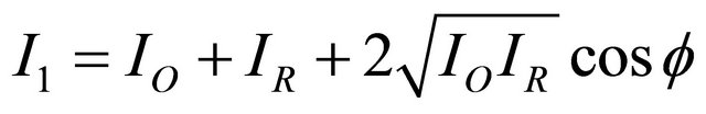 (1)
(1)
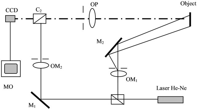
Figure 1. Experimental set-up for simultaneous opticalelectrochemical monitoring of corrosion processes.
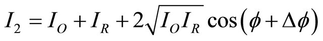 (2)
(2)
where f is the phase change between the object and reference beams, and Df (Df = (2p/l). The phase change is caused by the deformation “d”.
The first two terms of Equations (1) and (2) are terms of noise they be removed from the final image. The third term represents the interference term, where the phase information concerning the deformation.
If the signals V1 and V2 (the output of the camera) are proportional to the intensity of the input image, the signal resulting from the subtraction (VS) is given by:
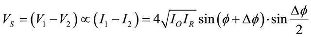 (3)
(3)
This signal has positive and negative values. Negative values are displayed as dark areas on the TV monitor. To avoid this loss of signal and obtain fringes, the square of the difference VS is running. Therefore the mean intensity at a given point B in the monitor image is:
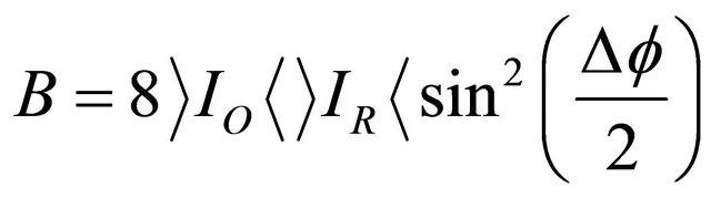 (4)
(4)
Equation (4) is similar to that obtained in conventional interferometry where the fringes are sinusoidally dependent on the phase difference to the deformation.
3. Results and Discussion
Presentation of the ideas here will be facilitated by a brief explanation of a dynamic cyclic polarization curve and its electrochemical regions associated to corrosion processes.
As an example, Figure 2 shows the initial interferogram at the beginning of the test and in used of schematic polarization curve diagram obtained for our cast steel sample immersed in salt water pH 1/4 4; in this graph different potential current density (oxidation-reduction) regions are observed and defined. 1) below the 500 mV potential is the cathodic region associated to reduction reaction processes where normal degradation of metal occurs; 2) above the same potential value an anodic
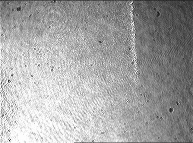
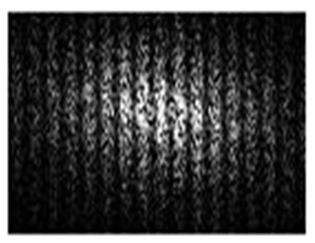
Figure 2. Displays the initial interferogram at the beginning of the test.
reaction region where active or general corrosion (oxidation) is generally favored and takes place is presented. The intersection of both branches at approximately 500 mV defines the open circuit or natural potential, where free corrosion conditions are presented and both anodic and cathodic reactions are in dynamic equilibrium. Afterwards, above the anodic branch at more positive potentials, a passive or corrosion products film formation region is revealed, where the presence of these corrosion products reduces the corrosion dissolution process or even more the corrosion rate (current density) becomes constant. The next region is the pitting potential located around 875 mV in Figure 2; from here on a new region, the transpassive one, defines the beginning of highly localized (pitting-type) corrosion processes.
The optical tool can be helpful as a technique complementary to the conventional ones for interpretation of some corrosion processes or electrochemical attack taking place at the metal-liquid interface, by analysis of the interference fringes evolution appearing through the polarization cycles during experimental tests.
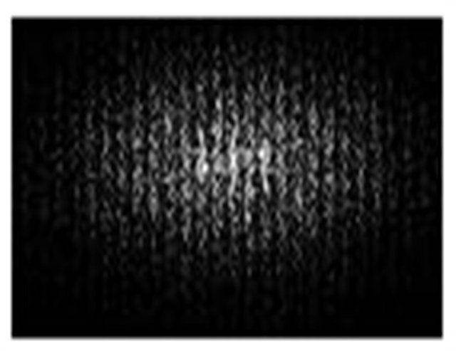
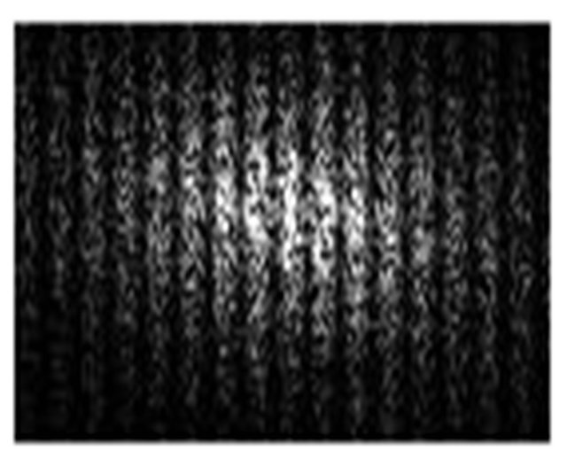
In Figures 3(a)-(f), consecutive interferograms obtained at each time interval on the corresponding polarization curve are displayed. While optical monitoring is performed one can clearly see how contrast of fringes diminishes rapidly as the intensity of current density is increased and practically, 30 s after polarization test had started such contrast seems to reach a minimum and remains at this minimum until the end of test (Figures 3(b)-(f)).
Furthermore, optical reflectance on cast steel surfaces is very low compared with that of stainless steel or copper, a property which avoids in this case any possible formation of interference processes.
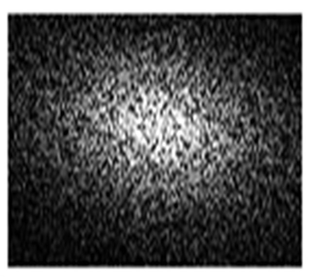
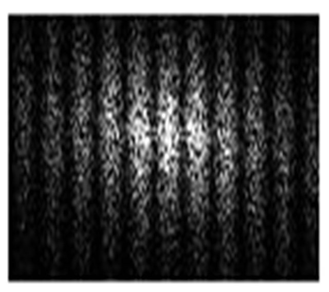
At first 3 min any important change on number or periodicity of fringes seems to be observed (Figures 4(a)- (c)), but during next 4 min an additional fringe appears on screen (Figures 4(d)-(f)) and during last 3 min. This behavior suggests an expected corrosion products film formation at an almost constant current density value of 8.0E_1 mA/cm2. By using the previously described model for anodic deposition in metals [5,6], and combining this with a commonly used electrochemical expression for calculation of corrosion-rate CR (usually expressed in mm/yr) proportional to the metal.
where n is the electrochemical valence, D is the density, K is a constant and a is the atomic weight of the electrode material (stainless steel). The current density diagram for the 304 stainless steel calculated by using the electro-chemical and optical methods separately. The first one is depicted by the continuous curve and has been evaluated as dependent on weight-gain calculated according to the data contained in.

(a) Specklogramm initial (b) Specklogramm taken after 5 min


(c) Specklogramm taken after 10 min (d) Specklogramm taken after 15 min

(e) Specklogramm taken after 20 min (f) Specklogramm taken after 25 min
Figure 3. Consecutive interferograms for a cast steel sample in salt water.
On the other hand, the blue dotted line shows the current density as depending on T and is calculated using N 1/4 3, l 1/4 632.8 nm and the following 304 stainless-steel physical parameters, n 1/4 2 electrons/ion, D 1/4 7.70 g/cm3, K 1/4 0.00327, and a 1/4 55.847 g/mol.
Below, we have plotted the contrast. For each aperture, we find a curve for the contrast when moving the object (sandpaper), another curve for the contrast related to the movement of the camera and finally, a curve for the ratio of these two contrasts (paper/camera).
But the point that interests us above all is γ. This is the fringe contrast.
Below we can see the result of approximation by Easyplot for two diaphragms. The curves correspond to a displacement of the object of 0.8 millimeters.
One can see that this approximation is good.
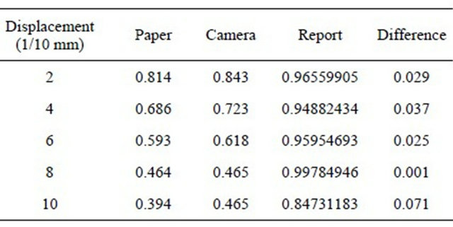
We have summarized the results of these approximations in the following tables, where we have only postponed the values of contrast (Tables 1 and 2).
Carry on the same graph the contrast ratio (paper/ camera) for the two stops. Do the same with the difference contrasts (camera/paper). We see that the ratio decreases more rapidly for the smallest opening, as well as the difference increases faster in this case (Figures 5-7).

(a) Specklogramm initial (b) Specklogramm taken after 5 min
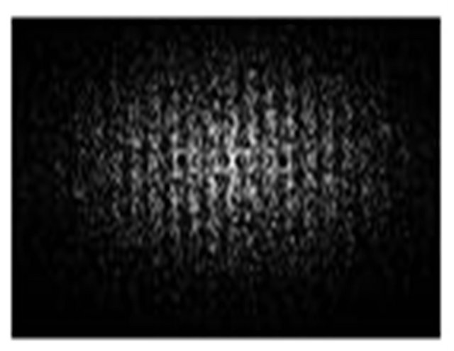
(c) Specklogramm taken after 10 min (d) Specklogramm taken after 15 min
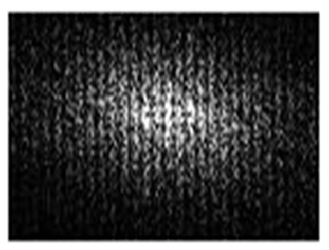
(e) Specklogramm taken after 20 min (f) Specklogramm taken after 25 min
Figure 4. Interferograms for a 304 stainless-steel sample immersed in distilled water and NaCl at 3% solution at: (a) 1 min; (b) 2 min; (c) 3 min; (d) 4 min; (e) 5 min; (f) 6 min after beginning of experimental test.
(a) Diaphragm 10.54 mm:
Table 1. Displacement of the diaphragm (10.54 mm).

(b) Diaphragm 2.63 mm:
Table 2. Displacement of the diaphragm (2.63 mm).
 (a)
(a)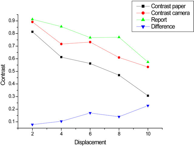 (b)
(b)
Figure 5. Contrast of an opening: (a) 10.54 mm; (b) 2.63 mm.
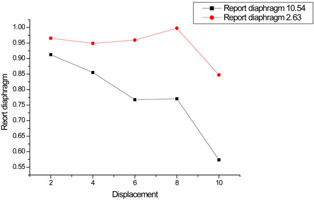
Figure 6. Contrast ratio for the two openings.
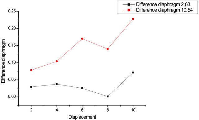
Figure 7. Difference in contrast to the two openings.
4. Conclusion
The experimental simultaneous combination of electrochemical and optical methods used here allows a close visual that follow up of the corrosion processes as well as their dynamics, giving as a result of a comparative analysis between obtained interferograms and the different polarization curves observed. The presented results show the advantages of using non-intrusive optical methods to help on interpretation and complementary corrosion indexes measuring, obtained by conventional electrochemical methods. Finally, the appearance/disappearance of interference fringes during optical monitoring of aluminum corrosion process in brine solution was also reported and briefly explained.
REFERENCES
- M. G. Fontana and N. D. Greene, “Corrosion Engineering,” 3rd Edition, McGraw-Hill, New York, 1986.
- P. Hariharan, “Optical Holography: Principles, Techniques, and Applications,” 2nd Edition, Cambridge University Press, New York, 1996. doi:10.1017/CBO9781139174039
- D. Mayorga-Cruz, P. A. Ma´rquez-Aguilar, O. SarmientoMartı´nez and J. Uruchurtu-Chavarı´n, “Evaluation of Corrosion in Electrochemical System Using Michelson Interferometry,” Optics and Lasers in Engineering, Vol. 45, No. 1, 2007, pp. 140-144. doi:10.1016/j.optlaseng.2006.02.001
- K. Habib, “In Situ Measurement of Oxide Film Growth on Aluminium Samples by Holographic Interferometry,” Corrosion Science, Vol. 43, No. 3, 2001, pp. 449-455. doi:10.1016/S0010-938X(00)00094-9
- K. Habib, “Model of Holographic Interferometry of Anodic Dissolution of Metals in Aqueous Solution,” Optics and Lasers in Engineering, Vol. 18, No. 2, 1993, pp. 115- 120. doi:10.1016/0143-8166(93)90016-E
- D. Mayorga-Cruz, J. Uruchurtu-Chavarı´n, O. SarmientoMartinez and P. A. Marquez-Aguilar, “Estimation of Corrosion Parameters in Electrochemical System Using Michelson Interferometry,” Proceedings of the 5th Symposium Optics in Industry, 10 February 2006. doi:10.1117/12.674445