Circuits and Systems
Vol.5 No.4(2014), Article ID:44856,16 pages DOI:10.4236/cs.2014.54012
Assigning Real-Time Tasks in Environmentally Powered Distributed Systems
Jian Lin1*, Albert M. K. Cheng2
1Department of Management Information Systems, University of Houston, Clear Lake, Houston, USA
2Department of Computer Science, University of Houston, Houston, USA
Email: *linjian@uhcl.edu
Copyright © 2014 by authors and Scientific Research Publishing Inc.
This work is licensed under the Creative Commons Attribution International License (CC BY).
http://creativecommons.org/licenses/by/4.0/


Received 19 January 2014; revised 19 February 2014; accepted 26 February 2014
Abstract
Harvesting energy for execution from the environment (e.g., solar, wind energy) has recently emerged as a feasible solution for low-cost and low-power distributed systems. When real-time responsiveness of a given application has to be guaranteed, the recharge rate of obtaining energy inevitably affects the task scheduling. This paper extends our previous works in [1] [2] to explore the real-time task assignment problem on an energy-harvesting distributed system. The solution using Ant Colony Optimization (ACO) and several significant improvements are presented. Simulations compare the performance of the approaches, which demonstrate the solutions effectiveness and efficiency.
Keywords:Distributed Systems, Energy Harvesting, Real-Time Scheduling, Task Assignment

1. Introduction
A distributed system consists of a collection of sub-systems, connected by a network, to perform computation tasks. Today, low energy consumption or green computing becomes a key design requirement for a lot of systems. Recently, a technology called energy harvesting, also known as energy scavenging, has received extensive attentions. Energy harvesting is a process that draws parts or all of the energy for operation from its ambient energy sources, such as solar, thermal, and wind energy, etc. As energy can be absorbed from a system’s ambient environment, it gives a low cost and clean solution to power the computer systems.
A real-time system provides a guarantee to complete critical tasks for responsiveness and dependability. Their operation must be completed before a deadline. An important category of real-time tasks is a periodic task in which a series of the task instance continuously arrive at a certain rate. When operating these tasks with energy harvesting, a concern of satisfying the timely requirement is raised. Operating computing tasks on a system consumes energy. To execute repeating, periodic tasks, a sustainable system must obtain energy not slower than it consumes energy. Otherwise, Figure 1 shows a scenario that a system with two periodic tasks running at a rate of 8 time units will ultimately crash or the task will finally miss its deadline due to the shortage of energy during run-time.
In this work, we study the scheduling of a set of real-time tasks on a distributed system powered by energy harvesting. We consider the static assignment in which each task needs to be statically assigned to a node before it executes. A feasible assignment can not violate the tasks’ deadline requirement and energy obtained from the node’s environment must be sufficient to run the tasks. The rest of the paper is organized as follows. In the next section, the related work is discussed. Then, we introduce the system model and problem definition in Section III. Section IV studies the solutions using Ant Colony Optimization (ACO). Also, we will show how to improve the ACO approach to adapt to an unstable environment. The simulation results are shown in Section V, and we conclude the paper in the last section.
2. Related Works
Scheduling computer tasks on a distributed system is a classical problem in computer science research. In the literature, many research results have been obtained without considering the energy issues. In [3] , a genetic algorithm based approach for solving the mapping and concurrent scheduling problem is proposed. In [4] [5] , the authors study the assignment problem for a set of real-time periodic tasks. The work in [6] gives a good survey and a comparison study of eleven heuristics for mapping a class of independent tasks. While assigning and scheduling a set of computer tasks, the above solutions are not suitable for considering the energy issue. Some research works find solutions for scheduling real-time tasks also looking into their energy consumption. For example, in [7] -[9] , a technique called Dynamic Voltage Scaling (DVS) is used to minimize the energy consumption. By adjusting the voltage of a CPU, energy can be saved while the execution of a computing task is slowed down. A common assumption is made in these works that the energy is sufficiently available at any time. Unfortunately, this assumption is not always true if the energy-harvesting approach is used. Recently, the energy-harvesting has been studied in a variety of research works. In [10] [11] , two prototypes are developed for systems to operate perpetually through scavenging solar energy. Lin et al. and Voigt et al. study clustering decisions within the network that the knowledge of the currently generated power is available at each node [12] . They show that the network lifetime can be optimized by appropriately shifting the workload. Energy-harvesting has also been discussed for real-time systems. A. Allavena et al. propose an off-line algorithm in [13] for a set of frame-based real-time tasks, assuming a fix battery’s recharge rate. Later, Moser et al. develop an on-line algorithm called lazy to avoid deadline violations [14] . Liu et al. improve the results by using DVS to reduce the deadline miss rate [15] . A new work for using the energy-harvesting is done in [16] that the Earliest Deadline First (EDF) scheduling algorithm has a zero competitive factor but nevertheless is optimal for on-line non-idling settings. All of the above works do not solve the scheduling problem on distributed real-time systems using energy harvesting, for which our solutions will be presented in the following sections.
3. Preliminaries
In this section, we describe the system model as well as the task model and power model. We also define the problem statement and discuss its complexity. We lastly introduce certain preliminary results for our problem.
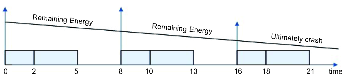
Figure 1. Consuming energy faster than energy harvested.
3.1. System, Task and Power Models
The task model of frame-based task used in [13] is adopted in this work. In this model, n real-time tasks must execute in a frame or an interval with a length L, and the frame is repeated. The frame-based real-time task is a special type of periodic system where every task in the system shares a common period p, . In each frame, all tasks are initiated at the frame’s beginning and must finish their execution specified by its computation time c by the frame’s end. For example, the task set shown in Figure 1 has two tasks and the frame’s length is 8 time units. Since all tasks start at the same time and share a common deadline in each frame, the order of executing these tasks in the frame does not matter which simplifies the scheduling decision. Also, a task consumes energy estimated by a rate of p when it executes. No energy consumption is assumed for a task if it is not in execution.
For the base system providing the computing power and energy, it is distributed and has m nodes. Each node is a complete system capable of executing real-time computer jobs, with an energy-harvesting device to generate energy. The m nodes are assumed to be located in different locations, and each has an estimated rate 
 of obtaining energy from their ambiance to be fed into the energy storage. We consider
  as a constant, but we relax this limitation in our later discussion. Each node has a storage device to store the energy. If the storage is full, continuing to harvest energy is just a waste and the excessive energy is discarded.
The system used can be homogeneous or heterogeneous. However, since the former one is just a special case of the latter one, we consider solving the problem on the heterogeneous systems. On a heterogeneous system, the computing speed and energy of running a task may be different for running on different nodes. What follows summarizes the parameters used in this paper:
m: the number of nodes.
n: the number of tasks in the frame-based application.
L: the frame’s length which equals to the period and relative deadline of every real-time task.
 : (recharge) rate of harvesting energy on node
 .
.
 : the computation time required to finish task i on node
 .
.
 : the overall power consumption rate for executing task i on node
 .
.
3.2. Problem Definition and Complexity
In statically partitioning the real-time tasks, a control system assigns the tasks to the nodes, and a task stays at a node during its lifetime after being assigned. In our later discussion, we also consider the cases that tasks can be reassigned if there is a change in the environment. Our goal is to determine the feasibility of the assignment on the system using energy-harvesting. The following definition formally defines the problem.
Definition 1: Energy Harvesting Assignment (EHA) problem, given a set of frame-based real-time tasks and an energy-harvesting distributed system specified by the parameters above, find a feasible assignment for the tasks such that:
a. Every task meets the deadline.
b. Energy remained in the storage of node j at the end of each frame interval is at least  where
where  is the initial level of the energy in the storage on node j.
Constraint a specifies the real-time requirement for completing the tasks. Constraint b guarantees that the energy harvested within each frame interval is not less than the energy consumed by running the tasks. When Constraint b is satisfied, the system is powered continuously and sufficiently for executing the repeating, frame-based tasks. Although all tasks in the application have the same starting time and deadline, the EHA problem is still an NP-Hard problem, even for a homogeneous system. For completeness, we give the proof of the following theorem for the homogeneous version of the problem. The proof of the heterogeneous version directly follows because it is a generalization of the homogeneous version.
Theorem 1: The EHA problem is NP-Hard.
Poof: we prove this theorem by performing a reduction from the 3-PARTITION problem which is known to be NP-Hard [17] to the EHA problem.
3-PARTITION: Given a finite set A of 3m elements, a bound , and a size
  for each
 such that each
  satisfies
  and such that
 . Question: Can A be partitioned into m disjoint sets
  such that, for
 ,
, ?
?
Suppose that an algorithm exists to solve the EHA problem, given the instance of the problem is feasible, in polynomial time. Given an instance of 3-PARTITION, we construct the instance of the EHA problem. The instance includes a set of 3m frame-based tasks and a system of m nodes. The length of the frame is B. The computation time of task i,  , equals to the size of
  in A. We assume that all nodes have the same recharge rate r, and all tasks have the same power consuming function
 , which means that the energy consumed by running the tasks is as fast as the energy harvested from the ambiance. Then, the shortage of the energy is not a concern. Also since
 , which equals the total length of the m frames, there is no idle interval in a feasible schedule because all CPU time must be used to execute tasks. If there is a solution for problem 3- PARTITION, we can apply the solution to our problem directly. If a feasible schedule exists for our problem, the length of the schedule in a frame on each node is exactly B because the schedules do not have any idle intervals. This is also the solution of the problem 3-PARTITION. The reduction is finished in polynomial time. Thus, if EHA problem can be solved in polynomial time, 3-PARTITON can be solved in polynomial time. However, this contradicts the known theorem that 3-PARTITION is NP-Hard. Thus, the EHA problem is NP-Hard.
3.3. Preliminary Results
In the EHA problem, if the constraint b is ignored, the feasibility after all tasks have been assigned on the system can be tested as:
 (1)
(1)
where  means the computation time of task i assigned on node j. If the energy issue is considered, A. Allavena et al. develop a schedulability condition in [13] for running a set of frame-based tasks on a single node system that has a rechargeable battery:
 (2)
(2)
In the inequality,  is an idle interval without any task execution, used for energy replenishment if the energy consumed for running tasks is faster than it is obtained from the environment. To calculate
 ,
,  , the energy’s instantaneous replenishment rate of the system while running task i, is calculated. Let
 .
.  means that running task i consumes energy slower than the system obtains energy and
  means the contrary. All tasks are then divided into two groups, namely the recharging tasks
  and the dissipating tasks
 . Two sums are calculated respectively, as
  and
and
 . In the equation,
  (or
(or ) is the amount of energy the system gains (or loses) while running the tasks in the group. The size of the idle interval is
 . We call this idle interval as recharging idle interval.
Let us extend (2) to the EHA problem and we have:
 (3)
(3)
where  means the computation time of task i assigned on node j. The inequality 3 can be used to replace the constraints a and b to determine the feasibility of an assignment instance of the problem. Due to the intractability, it is not likely to find a feasible assignment for every instance in polynomial time. In the following sections, we will discuss the approaches to solve the problem.
4. ACO Solution
The ACO algorithm is a meta-heuristic technique for optimization problems. It has been successfully applied to some NP-Hard combinatorial optimization problems. In this section, we apply and improve the ACO for our EHA problem. Before we describe our approach, we briefly introduce ACO meta-heuristic. The readers who are familiar with the ACO can skip the introduction in subsection A.
4.1. Basic ACO Structure
The ACO algorithm, originally introduced by Dorigo et al., is a population-based approach which has been successfully applied to solve NP-Hard combinatorial optimization problems [18] . The algorithm was inspired by ethological studies on the behavior ants that they can find the optimal path between their colony and the food source, without sophisticated vision. An indirect communication called stigmergy via a chemical substance, or pheromone left by ants on the paths, is used for them to look for the shortest path. The higher the amount of pheromone on a path, the better the path it hints, and then the higher chance the ant will choose the path. As an ant traverses a path, it reinforces that path with its own pheromone. Finally, the shortest path has the highest amount of pheromone accumulated, and in turn it will attract most ants to choose it. The ACO algorithm, using probabilistic solution construction by imitating this mechanism, is used to solve NP-Hard combinatorial optimization problems.
1) initialization (parameters, pheromone trails)
2) while true do 3) Construct solutions;
4) Local search;
5) Update pheromone trails;
6) Terminates if some condition is reached;
7) end Algorithm 1: ACO Algorithm’s Structure In general, the structure of ACO algorithms can be outlined in Algorithm 1. The basic ingredient of any ACO algorithm is a probabilistic construction of partial solutions. A constructive heuristic assembles solutions as sequences of elements from the finite set of solution components. It has been believed that a good solution is comprised by a sequence of good components. A solution construction is to find out these good components and then add them into the solution at each step. The process of constructing solutions can be regarded as a walk (or a path) of artificial ants on the so called construction graph. After a solution is constructed, it is evaluated by some metric. If the solution is a good solution compared with other solutions, a designated amount of pheromone is added to each component in it which will make the components to be a little bit more likely selected in next time of construction of solution. Components in good solutions accumulate probability of being selected in iterations and finally the selections will converge into these good components. This process is repeated until some condition is met to stop.
4.2. ACO for EHA Problem
In order to apply the ACO to the EHA, we see the EHA problem as an equivalent optimization problem. The following definitions define the metric used in the optimization problem.
Definition 2: Energy and Computation Time Length (EC-Length), the EC-Length of a node j is defined as the total computation time plus the  for the tasks assigned on that node.
Definition 3: Energy and Computation Time Makespan (EC-Makespan), Given an assignment, the EC-Makespan denotes the maximum value of the EC-Length upon all nodes.
The objective in our ACO system is to minimize the EC-Makespan. The task set is schedulable only if it can find an assignment in which the minimum EC-Makespan is not larger than the frame’s length L.
Initialization: At the beginning, the values of the pheromone are all initialized to a constant . In [19] , a variation of the original ACO algorithm called Max-Min Ant System (MMAS), was proposed to improve the original ACOs performance. The intuition behind the MMAS is that it addresses the premature convergence problem by providing bounds on the pheromone trails to encourage broader exploration of the search space. We dynamically set the two bounds in our system according to current best solution as in [19] .
Construct solutions: The solution component treated in our approach is the (task, node) pair. A chessboard can be used as the construction graph. Table 1 gives an example of 4 tasks and 3 nodes. In that example, ants traverse the chessboard by satisfying: One and only one cell is visited in each row; Constraints a and b must be respected. For each ant at a step, it first randomly selects a task, and then selects a pair of the  to be added into the solution according to the probabilistic model (4):
 (4)
(4)

Table 1. An example of the chessboard.
where  is the set of next possible move of the ant to assign task i. In 4,
  denotes the amount of pheromone which shows the quality of assigning task i to node j by the past solutions. The
  is a local heuristics defined as 1/current EC-Makespan. The current EC-Makespan is the one after task i is assigned to node j, evaluated by a heuristic. This local heuristic gives preference to the move with the possibly smallest EC-Makespan based on the currently completed, partial solution. The use of
  and
and  is to avoid the convergence too early either into the assignments of the completed solutions or to the looked-like good selections evaluated by a local heuristic. The α and β are parameters to control the relative importance between
  and
and . We assign 0.5 to each of them to make
  and
and  equally important. After all ants finish the construction of solutions, we check the final EC-Makespan. If the final EC-Makespan is not larger than L, the solution is identified as feasible, or infeasible, otherwise.
Local Search: To further improve the solution found by ACO, a local search optimization is performed on the infeasible solutions found by ACO. The local search in our problem tries to balance the load on different nodes. In our approach, we first find the most heavily loaded node, i.e., the node that contributes the final EC-Makespan, from which we try to reduce its load by moving some tasks to other lightly loaded node. The move is made only if the new final EC-Makespan does not exceed the old one. To reduce the time cost, at most 2 tasks are tried on the balanced node for local search. In our experiments, the performance of our ACO approach can be greatly improved with the local search.
Pheromone updates: In an iteration, ants deposit pheromone according to the quality of those solutions they find. A straight-forward definition of the quality is the EC-Makespan. The amount of the pheromone deposited is set to be 1/ EC-Makespan. A general formula to update the pheromone at the  iteration is given in (5):
 (5)
(5)
where . The rule increases the amount of the pheromone on the components in the solutions constructed by the ants, according to the solutions’ quality. The
  is called evaporation rate to decrease the amount of all pheromone trails at each iteration, to avoid an early convergence. In MMAS, only the best one in the m ants is allowed to deposit pheromone after an iteration, and this strategy has been reported to achieve better performance. In the completed solutions, the local best is the best one completed by the ants in the current iteration, and the global best is the best one in all of the completed solutions. The work in [19] suggests a mixed scheme which has shown performance better than average: either the local best or the global best is used.
Stopping conditions: ACO is a search-oriented approach. We do not want it to run infinitely in any way. In the problem of finding the minimum EC-Makespan, a value of a variable is used to monitor the number of iterations for which the performance is not improved. The variable, called , is initialized to 0. In each round, if the local best solution is not better than the global one, the value is increased by 1. The algorithm stops when
  reaches a threshold. Or, the algorithm stops when at least one feasible solution is found, for the original EHA problem.
4.3. MACO for Multiple Resources Constrained Assignment Problem
In ACO, using a local heuristic acts as it guides the ants to explore the solution space that is more likely to contain the optimal solution. However, is the guiding by the heuristic always in a correct direction? In EHA problem, there are two constraints, time and energy, and each constraint denotes the requirement of a single resource dimension. In most cases we do not have the knowledge a priori about how the resources are constrained in a given system. The local heuristic 1/current EC-Makespan, composed by the recharging idle interval and the sum of execution times of the tasks, seems good to the cases where energy and time are constrained evenly. However, in some cases, energy can be much more constrained than time, and vice versa. Then, using 1/current EC-Makespan as the heuristic may lead ants in a wrong direction. Due to the difficulties of analyzing the intrinsically constrained extent of different resources in a system, using a single heuristic is not likely to work well in all circumstances. While ants are guided in a wrong direction, stagnation on non-optimal solutions will be very likely to happen.
A novel structure called Multi-heuristics ACO (MACO) is proposed to solve the problem mentioned above. In ACO, only one group of ants is sent to search solutions by using a single heuristic. In MACO, however, we can distribute the ants into multiple groups for doing the search in different directions. Each group has its own used heuristic and independent pheromone trail. For our problem, three groups are defined, namely EC ants, energy ants, and time ants. While the EC ants use the same composite heuristic as the one in our original ACO algorithm, the energy ants (or time ants) has a heuristic in energy (or time) dimension. Two good options for the heuristic are 1/(energy requirement) and 1/(execution time accumulation). The former one prefers a low energy requirement for completing a task on a node (which is ). The latter one wants a selection with a small computation time.
1) In the first step, M ants are divided into  groups using
  hruristics (m dimentional heuristics and n composite heuristics), evenly or not evenly. Apply the ACO algorithm to each group independently. After certain iterations, the best k groups are selected to be used in the second group.
2) In the second step, M ants are placed into the k groups, evenly or not evenly. Apply the ACO algorithm on each group independently. The best result among the group(s) is used as the solution.
Algorithm 2: Two-Step MACO.
4.4. Two-Step MACO
When using the same number of ants, MACO could perform worse than ACO in some cases. This is because when the composite heuristic used in ACO happens to be the right one, MACO has fewer ants working in the correct direction. To solve this problem, we use a two-step, or an incremental method, called coarse and fine searching. In the first step, a small number of ants are sent in different directions guided by the heuristics for a certain number of iterations. After that, we calculate the global best for each group. The best global solution indicates a correct direction. In the second step, all ants using the heuristic of the best group research the solution space for finding the optimal solution. This process can be seen as the cooperation between detective ants and worker ants. The detective ants do the coarse search, and then the worker ants search the space deeply that is most likely to contain the optimal solution (reported by the detective ants). The rationale behind the technique has two folds. The first one is the exploration, where a good searching direction shown in the coarse search is more likely to be the right one. The second one is the exploitation, in which good solutions are normally “close” to each other. The two-step MACO framework is described in Algorithm 2.
4.5. ACO for Changing Environments
The recharge rate of a node is estimated for a period of running the application. In some cases, the environment where a node is located is not stable, we must consider the impact brought by the fluctuating rate of obtaining ambient energy. Imagine that a feasible assignment has been made on a distributed system using solar energy. Later, in one of the places where a node locates, the sky becomes suddenly covered by dark clouds. This situation unavoidably results in a lower rate of the energy’s replenishment to the system. According to our previous discussion, this decreased recharge rate requires a longer recharging idle interval, which may cause the tasks assigned on the node to miss their deadline. One possible solution to this problem is to keep executing the tasks in each frame and holds a hope that the sunny day will come back soon. This gambling manner, however, faces a risk that the system may ultimately crash due to the continuously decreasing energy level. Another possible solution is to reconfigure the assignment of tasks as quickly as possible.
In ACO, good solutions normally share common components and related to each other. For designing a fast algorithm which quickly adapts to changes, instead of re-constructing a new system of pheromones, it is beneficial to keep and use the useful knowledge saved in the old pheromones, and take into account where the changes occur. In our problem, the concern is when the nodes may experience a decreased recharge rate. When the feasibility of tasks assigned on a system might fail due to a change in the recharge rate, we should move the tasks with a high energy-demand to another node. A reasonable way to update the pheromone table is to reduce the amount of the pheromone of a high energy-demand task to the node. Suppose that the node is j. The following formula gives the rule to update the pheromone trails for the node.
 (6)
(6)
In 6, the pheromone on every path from a task to node j is updated. The old pheromone value is timed by a ratio to obtain its new value. The ratio is determined by the ratio of the task’s energy requirement if executed on j, and the total energy requirement of all tasks if executed on j. The higher the ratio, the larger the pheromone’s amount decreases, which in turn makes the larger energy-demand task less likely to be assigned on j. After the updates on the pheromone table finish, an ACO system using the updated pheromone values is executed to find a new feasible solution. If a small change, there is no need to re-search the correct direction by using the MACO.
5. Performance Results
In this section, we compare the performance of the proposed algorithms using extensive simulations. EC-Makespan is the key factor to determine the schedulability. An algorithm capable of obtaining a small EC-Makespan can achieve a high feasibility. Hence, we use the average EC-Makespan as our main performance metric to compare the algorithms. In our experiments, another meta-heuristic search method, Genetic Algorithm (GA), is also used to generate solutions. The GA algorithm we use is an implementation of the one in [3] . Also, two heuristics named MEC and MmEC proposed in our previous works [1] [2] which are two extensions of the list scheduling, are used for comparisons. The parameters used in these approaches are set to be relatively large to allow them to converge.
5.1. Simulation Settings
The main parameters of a frame-based real-time task are its computation time and frame length. Because we use the minimum EC-Makespan as the performance metric, the frame length is not used. We assume that the tasks’ computation times in a set range from 3 to 20 time units. The largest task runs nearly 7 times longer than the smallest task. Another important characteristic of a task in our experiments is its power characteristic. A broad range of the relative values between a task’s discharge rate and the system’s recharge rate is used. We assume that the recharge rate has a broader range because in the extreme cases a system obtaining energy can be very slow or pretty fast, compared with consuming energy for running tasks. An even distribution of probabilistic model is used to generate the computation time, recharge rate and discharge rate, randomly. Also, we assume that the number of nodes in a distributed system is 8 and the numbers of tasks are 40, 50, …, 90. The workloads are adjusted by using the different numbers of tasks in the experiments. Table 2 summarizes the parameters we mentioned in this paragraph.
Table 3 and Table 4 give the parameters we use for the ACO approach and GA approach. In the GA approach, a chromosome sequence encodes an assignment solution of the EHA problem. The fitness value is the EC-Makespan of assignment. For a fair comparison, we use the same local heuristic MmEC in both meta-heuristic approaches. Also, they use the same stopping condition that the number of no improvement iterations is 30. There is another stopping condition required by the GA approach which is the number of total iterations. We set it to be 1000 to allow it large enough to converge. The simulations are performed by adjusting simulation parameters. Each time, 100 task sets are generated randomly. For each approach, we record the values of EC-Makespan and execution time of running the algorithm. The average results are used to evaluate and compare the performances.
5.2. Results on Different Circumstances
The computing resources, such as the CPU time and the available amount of energy, may not be necessarily evenly-constrained for running a set of tasks. The main purpose of designing the MACO approach is to give adaptiveness to ACO for working well in different circumstances. Hence, we perform the simulations mainly in the following categories: resources evenly constrained, tightly energy-constrained and time-constrained.
Table 2. Simulation parameters.
Table 3. ACO/MACO parameters.
Table 4. GA parameters.
Category 1: The simulations done in this category has set the parameters to be timing and energy evenly constrained. To accomplish this, we select a node’s recharging function between 4.0 and 7.0, and then select a task’s discharging rate from 2.0 to 9.0, randomly. By using an even distribution, both the recharge rate and discharge rate have an expected value of 5.5 which means in average the numbers of recharge tasks and dissipation tasks are equal. The workload is changed by adjusting the number of tasks in the task set.
Figure 2 shows the average EC-Makespan measured for the used approaches. In the figures, when the number of tasks is less than 75, ACO and MACO outperform the other approaches. When the number of tasks is 75 or larger, ACO and MACO are not as good as GA and MmEC. However, by analyzing the results, we found that GA, which builds its solution upon MmEC, has almost the same performance as its seed. This implies that GA does little to improve MmEC and its performance is sticky with MmECs. It has been well known that when the size of a problem instance is large and if the number of agents is not enough, the performance of using meta-heuristics degrades because the probabilistic selecting process is not significant. The solution for the degradation is straight-forward as increasing the number of ants. Also, it is not a surprise that ACO and MACO perform very close for reducing the EC-Makespan in this category. This is because the composite heuristic used by ACO happens to be the correct heuristic found by the detective ants in MACO. In Figure 3, the execution times of running ACO, MACO and GA are compared. ACO uses less time than GA in the cases of having less than or 75 tasks. It implies that if given the same time cost the ACO approach will outperform the GA approach.
Category 2: The simulations in this category are set to be tightly energy-constrained. The recharging rates are selected from a low range [1.0 6.0], implying that the systems need longer time to refill energy. The tasks’ power consuming rates are selected from a high range [5.0 9.0], which makes more tasks as dissipating tasks. We also reduce the execution times for tasks by dividing them with a number in [4.0 5.0] to make the system truly energy constrained. Figure 4 illustrates the results that the MACO has the best performance. In the figures, MACO always defeats ACO in the performance of reducing the EC-Makespan. When the system is energy tightly constrained, the energy-oriented heuristic leads the ants to find the optimal solutions. The results support the effectiveness of using our MACO strategy that it gives adaptiveness to the original ACO approach. Figure 5 shows the execution times for running the algorithms. The execution time for running MACO is about twice of running ACO.
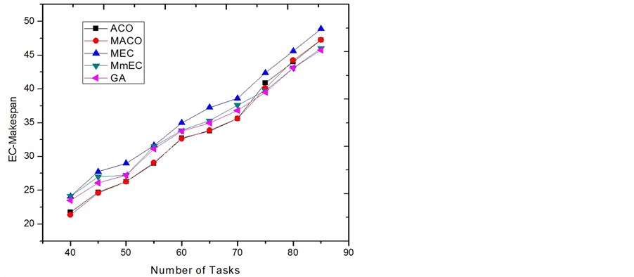
Figure 2. EC-Makespan comparison of category 1.
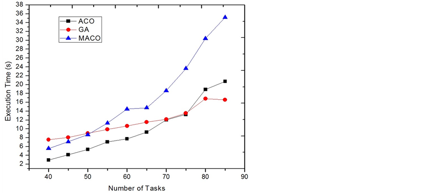
Figure 3. Execution time comparison of category 1.
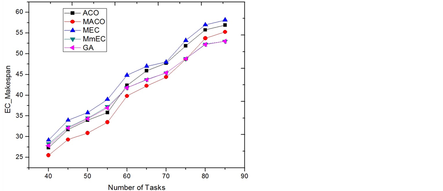
Figure 4. EC-Makespan comparison of category 2.
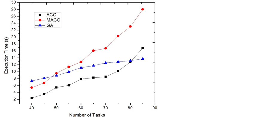
Figure 5. Execution time comparison of category 2.
Category 3: In this category (Figure 6 and Figure 7), the power consumption rates for most tasks ([2.0, 6.5]) are set to equal or smaller than the recharging rates ([6.0, 12.0]). When the system is only timing constrained, MACO outperforms ACO and other algorithms due to its unique adaptability.
When we compare our ACO approaches with the GA approach, we use different values for the crossover rate and mutation rate. The results are similar to the result shown in the three categories.
5.3. Two-Step MACO
We proposed a two-step MACO solution for the problem but one might ask a question: why uses two-step ACO? Why not just placing more ants in each direction to search the optimum? We answer this question by showing the result of the following simulations for three different implementations of MACO on a small-sized input.
a. One-step MACOm. In this approach, there are 3 ants and 3 groups, each group has 1 ants. The optimal solution is the best solution found in the three groups.
b. One-step MACO3m. In this approach, there are 9 ants and 3 groups, each group has 3 ants. The optimal solution is the best one found in the three groups.
c. Two-step MACO2S. This is the one we proposed to do the coarse and fine search. There are 3 groups of ants used for the two steps, respectively. In the first step, each group has 1 ant. In the second step, 3 ants are used in the selected group.
The implementations for a and b are both one-step MACO, in which b has 2 more ants than a. in each group or direction. The implementation c uses only 1 ant in each group in the coarse stage, but uses 3 ants to search space in the reportedly correct direction. The total number of the ants used in each approach is 3, 9, and 6, respectively.
Figure 8 and Figure 9 give the results on EC-Makespan and execution times for the three MACO implementations. It can be seen that b and c both improve the result of one-step MACO with small number of ants, on EC-Makespan. Also, the results of b and c are almost the same as shown in Figure 8. This implies that for two-step MACO, even though the number of detective ants in each group is 1, the correct direction for doing the fine searching can still be found. For the execution time, however, b uses about 1/3 more time than c. It is not hard to conclude that our two-step MACO approach finds a reasonable way to handle the trade-off between the performance and the time cost.
5.4. Dynamic ACO
In a previous section, we showed how to update the pheromones in order to make the system quickly adaptable to changeable environments. In this section, we show the method’s effectiveness. In the simulations, we first use two-step MACO to obtain the minimum EC-Makespan for assigning a task set on the 8 nodes. Next, one of the nodes is randomly chosen to decrease its recharge rate. We compare the approaches Complete Restart and
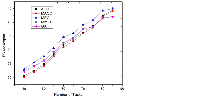
Figure 6. EC-Makespan comparison of category 3.
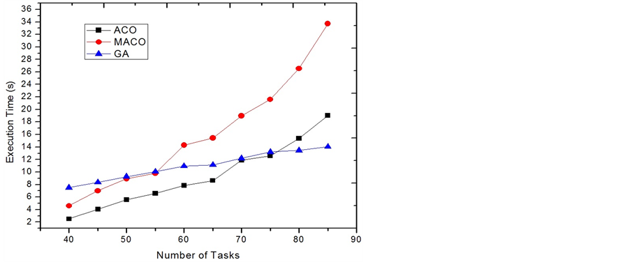
Figure 7. Execution time comparison of category 3.
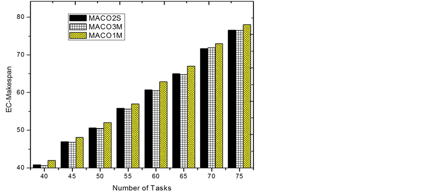
Figure 8. EC-Makespan comparison of MACO.
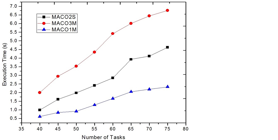
Figure 9. Execution time comparison of MACO.
Dynamic ACO by calculating the new minimum EC-Makespan. While the Complete Restart is just simply restarting a new ACO process, Dynamic ACO modifies and utilizes the known knowledge stored in pheromones to find the new solution. At the beginning, we assume that only one node experiences an environment change. Figure 10 and Figure 11 show the comparisons of the normalized EC-Makespan and running time between the two approaches. In the figures, the numbers on the x axis are labeled as the extent of the decreased rate of obtaining energy. For example, if before a change the recharge rate of the system is r, 50% means that the new recharge rate becomes  after the change. It can be seen that with using around 50% less time, Dynamic ACO slightly outperforms Restart. This is because in these simulations only a small change occurs, most components with high pheromones are still good components for the new solution. Therefore, searching solution using the pheromones after a small and appropriate modification in fact acts as a deeper and broader search with a right direction. On the contrary, approach Restart totally discards the useful known-knowledge and simply carries on the work again. While they both have the same stopping criteria and correct direction to search, Dynamic ACO starts ahead of Restart and actually does a deeper exploration. We also compare the two approaches according to the number of nodes having a change in recharge rate. Figure 12 and Figure 13 show the results based on five groups. In each group, a specific number of nodes are randomly chosen to lower down their recharge rate 50%. It can be seen that when the number of changes is equal to or larger than 5, the running time of Dynamic ACO is close to doing Restart. However, its result on reducing EC-Makespan becomes worse. This is because when a large number of changes occur, the information stored in the pheromones becomes stale. To keep using the stale information to search solutions normally makes the search to go in a wrong direction. In these situations, Restart seems a more appropriate way to find the optimal solutions.
6. Summary and Future Works
In this paper, we consider a real-time task assignment problem for an energy-harvesting distributed system. We focus on the ACO approach and its improvements such as MACO and Dynamic ACO. The experimental results show that our proposed algorithms work effectively and efficiently. The MACO improvement provides a good adaptability in our EHA problem. It not only gives good results, but also gives a suggested framework to solve the multi-resources constrained problems using ACO. The Dynamic ACO is used to search a new solution when a small change happens to the data set of the problem. It is believed that if the change is not significant, there is no need to start a new search over. Most of knowledge stored in the original pheromones can be used without a big modification to the pheromones. This way reduces the time cost significantly for searching a new solution upon a change. In the future, our works may include solving problems with various QoS requirements when assigning real-time tasks on a distributed system. While some sorts of QoS are required, the problem set becomes
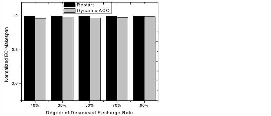
Figure 10. EC-Makespan comparison for a single node change.
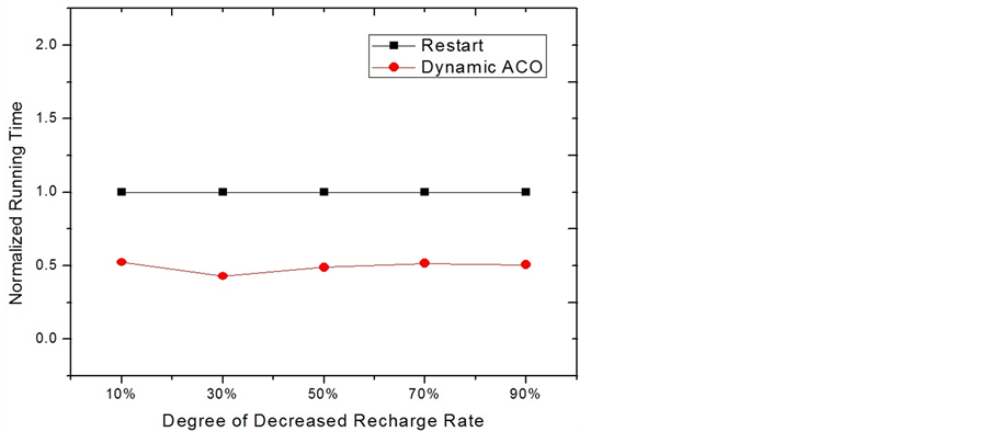
Figure 11. Execution time comparison for a single node change.

Figure 12. EC-Makespan comparison for multi. node change.
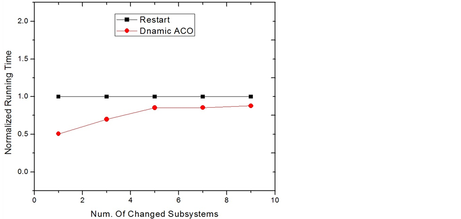
Figure 13. Execution time comparison for multi. node change.
more complicated. Also, we may look at a more complex model for the tasks, such as considering input/output activities. Dependent task model can be studied as well. Both of these problems definitely give another challenge.
References
- Lin, J. and Cheng, A.M.K. (2008) Real-Time Tasks Assignment in Rechargeable Multiprocessor Systems. Proceedings of IEEE-CS International Conference on Embedded and Real-Time Computing Systems and Applications, Kaohsiung, 25-27 August 2008, 279-284.
- Lin, J. and Cheng, A.M.K. (2009) Real-Time Task Assignment in Heterogeneous Distributed Systems with Rechargeable Batteries. Proceedings of IEEE-CS International Conference on Advanced Information Networking and Applications, Bradford, 6-29 May 2009, 82-89.
- Wang, L., Siegel, H.J., Roychowdhury, V.P. and Maciejewski, A.A. (1997) Task Matching and Scheduling in Heterogeneous Computing Environments Using a Genetic-Algorithm-Based Approach. Journal of Parallel and Distributed Computing, 47, 8-22.
- Funk, S. and Baruah, S. (2005) Task assignment on Uniform Heterogeneous Multiprocessors. Proceedings of the 17th Euromicro Conference on Real-Time Systems, 6-8 July 2005, 219-226. http://dx.doi.org/10.1109/ECRTS.2005.31
- Baruah, S.K. (2004) Partitioning Real-Time Tasks among Heterogeneous Multiprocessors. Proceedings of the 2004 International Conference on Parallel Processing, 15-18 August 2004, 467-474.
- Braun, T.D., Siegel, H.J. and Beck, N. (2001) A Comparison of Eleven Static Heuristics for Mapping a Class of Independent Tasks onto Heterogeneous Distributed Computing Systems. Journal of Parallel and Distributed Computing, 61, 810-837.
- Luo, J. and Jha, N.K. (2007) Power-Efficient Scheduling for Heterogeneous Distributed Real-Time Embedded Systems. IEEE Transactions on Computer-Aided Designs of Integrated Circuits and Systems, 26, 1161-1170.
- Mishra, R., Rastogi, N., Zhu, D., Mosse, D. and Melhem, R. (2003) Energy Aware Scheduling for Distributed RealTime Systems. International Parallel and Distributed Processing Symposium. http://dx.doi.org/10.1109/IPDPS.2003.1213099
- Kumar, G., Manimaran, G. and Wang, Z. (2008) End-to-End Energy Management in Networked Real-Time Embedded Systems. IEEE Transactions on Parallel and Distributed Systems, 19, 1498-1510. http://dx.doi.org/10.1109/TPDS.2008.124
- Raghunathan, V., Kansal, A., et al. (2005) Design Considerations for Solar Energy Harvesting Wireless Embedded Systems. Proceedings of the International Symposium on Information Processing in Sensor Networks, 15 April 2005, 457- 462.
- Jiang, X., Polastre, J. and Culler, D.E. (2005) Perpetual Environmentally Powered Sensor Networks. Proceedings of the International Symposium on Information Processing in Sensor Networks, Piscataway.
- Lin, L., Shroff, N.B. and Srikant, R. (2007) Asymptotically Optimal Power-Aware Routing for Multihop Wireless Networks with Renewable Energy Sources. ACM/TEEE Transactions on Networking, 15.
- Allavena, A. and Mosse, D. (2001) Scheduling of Frame-Based Embedded Systems with Rechargeable Batteries, in Workshop on Power Management for Real-Time and Embedded Systems (In Conjunction with RTAS 2001).
- Moser, C., Brunelli, D., Thiele, L. and Benini, L. (2006) Real-Time Scheduling with Regenerative Energy. Proceedings of the Euromicro Conference on Real-Time Systems, Dresden, 2006, 10-270. http://dx.doi.org/10.1109/ECRTS.2006.23
- Liu, S., Lu, J., Wu, Q. and Qiu, Q. (2012) Harvesting-Aware Power Management for Real-Time Systems with Renewable Energy. IEEE Transactions on Very Large Scale Integration (VLSI) Systems, 20, 1473-1486.
- Chetto, M. and Queudet, A. (2013) A Note on EDF Scheduling for Real-Time Energy Harvesting Systems. IEEE Transactions on Computers, 63, 1037-1040.
- Garey, M. and Johnson, D. (1979) Computers and Intractability: A Guide to the Theory of NP-Completeness. Freeman, New York.
- Dorigo, M. and Stutzle, T. (2004) Ant Colony Optimization. MIT Press. http://dx.doi.org/10.1007/b99492
NOTES

*Corresponding author.